
- SAP Community
- Products and Technology
- Technology
- Technology Blogs by SAP
- Extending SAC Planning – Creating custom calculati...
Technology Blogs by SAP
Learn how to extend and personalize SAP applications. Follow the SAP technology blog for insights into SAP BTP, ABAP, SAP Analytics Cloud, SAP HANA, and more.
Turn on suggestions
Auto-suggest helps you quickly narrow down your search results by suggesting possible matches as you type.
Showing results for
Product and Topic Expert
Options
- Subscribe to RSS Feed
- Mark as New
- Mark as Read
- Bookmark
- Subscribe
- Printer Friendly Page
- Report Inappropriate Content
05-22-2023
8:07 AM
Learn how a SAC Planning model can be populated with data coming from custom calculations or Machine Learning. We describe this concept in a series of three blogs:
This diagram shows the architecture and process from a high level:
The whole concept and blog series has been put together by maria.tzatsou2, andreas.forster, gonzalo.hernan.sendra and vlad-andrei.sladariu.
In the previous blog it was explained, how to capture input from the planning user and how to expose this information in the backend as Remote Table in SAP Datasphere. In this blog we will use that data in a very simple custom calculation example. We train a Machine Learning model (regression) to learn from a product's past, how the price that we charged (UnitPrice) correlates to the quantities we sold (UnitsSold). This model is then applied on the prices we intend to charge in the coming months to estimate the sales quantities we can expect each month.
The same architecture and concept can be used for more complex requirements. You have access to a very comprehensive Machine Learning library with 100+ algorithms. For example we have used this concept to add a risk assessment to SAC Planning by integrating Monte Carlo simulations. The Monte Carlo topic could be worth a separate blog, let us know, if you would find this valuable.
We are using the Machine Learning that is embedded in SAP Datasphere / SAP HANA Cloud to avoid data extraction to keep the architecture lean. This is possible, as the built-in Machine Learning frameworks PAL (Predictive Analysis Library) and APL (Automated Predictive Library) can work with the planning data.
SAP Datasphere includes besides the Machine Learning frameworks also other analytical engines like geospatial or text analysis. Since all these engines are built into SAP Datasphere / SAP HANA Cloud, they work directly on the data without having to extract the content elsewhere.
In this blog we use Python to trigger the Predictive Analysis Library. This is possible thanks to our hana_ml package, which provides a convenient option to trigger those engines out of your favourite Python environment. This means you can remain in your familiar interface to trigger the algorithms on your planning data in this case. Personally, I prefer to script Python in Jupyter Notebooks, but you can use the environment of your choice.
For an introduction on this package and how to use it with SAP Datasphere, please see the previous blog in this series. In this very blog, we assume you have some familiarity with that package and only mention the most important steps needed for the SAC Planning extension. All necessary code is listed in this blog, but you can also download the actual files from the samples repository.
To work with Jupyter Notebooks you can install for example Anaconda. In the "Anaconda Prompt" type "jupyter lab" to open the notebook environment. Install the hana_ml package with
Connect to SAP Datasphere from Python. This requires:
When your system has been configured, you can test establishing a connection from your local Jupyter notebook with logon credentials in clear text.
If this succeeds, you can use the SAP HANA User Store to keep the credentials in a safe place, to avoid having to use a password in clear text. If you would like to set this up, please see the bonus section at the bottom of this blog.
To start working with the data, create a hana_ml Dataframe, that points to the view, that accesses the user input. This is the view, which was created in the previous blog (ie "ExtSACP01_FactData_View"). To improve calculation performance save the data into a temporary table in SAP Datasphere, here called "#PLANNINGDATA". All data is staying in the cloud. Just display a few rows to verify that the data is available.
First we train a simple Machine Learning model on the actuals data, to use the UnitPrice as Predictor to explain the UnitsSold. This requires some semantical data transformation. In the original structure these two values that belong to the same months (UnitPrice and UnitsSold) are spread across two rows of data. Structure the data, so that both values for the same month become columns for the same row. Display a few rows to verify the output.
Similarly, prepare the data on which the model will be applied to estimate future sales quantities. We use the planned UnitPrice for the months, for which no actuals are available yet (April to December 2023 in this example).
Trigger the training of the Machine Learning model, using the embedded Machine Learning in SAP Datasphere. We use a simple linear regression.
We are not testing the model further. Let's just have a quick look at the model quality. An R'2 of 0.96 shows that the model describes the relationship between UnitPrice and UnitsSold extremely well. We are using sample data. Should your own models on real data come with similar statistics, you may want to be suspicious that something went wrong.
Now apply the trained model to predict the UnitsSold for the future months, based on the planned UnitPrice for each month. The prediction itself is just one line of code. The remainder of the code structures the data to be in the necessary format so that SAC Planning can import it later on.
And save those predictions to a physical table in SAP Datasphere, from where SAC Planning can import the data.
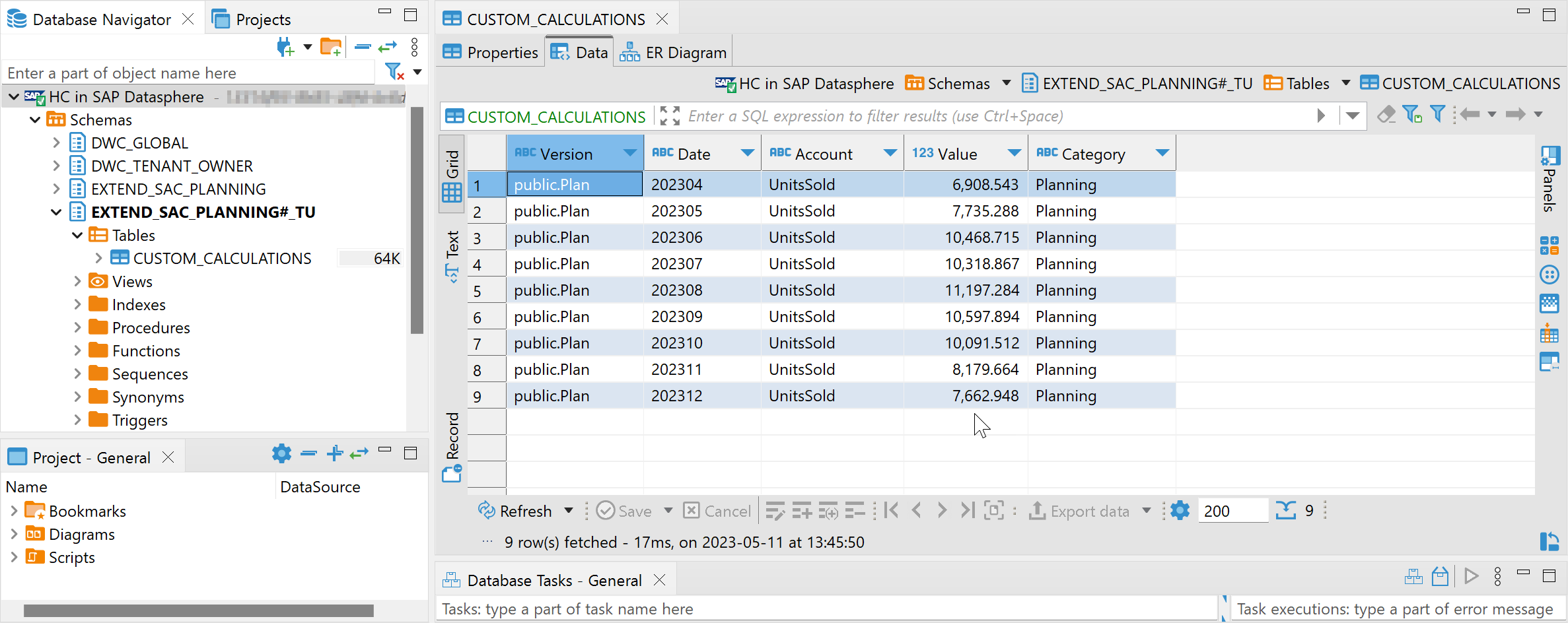
You can now see the forecasts in the table, for example via the SAP HANA Database Explorer or in tools like DBeaver.
Once we are happy with the code from the Jupyter Notebook, it needs to be callable via REST-API, to be integrated into the SAC Planning workflow. For the deployment of that Python code you can use any environment that is able to expose such code as REST-API, for instance Cloud Foundry, Kyma or SAP Data Intelligence.
In this example we use Cloud Foundry, which is a very lightweight deployment on the SAP Business Technology Platform. In case you haven't deployed Python code yet on Cloud Foundry, you can familiarise yourself with the blog Scheduling Python code on Cloud Foundry. In our case however, we don't need to schedule any code, hence you can ignore that part of the blog. You do not need to create instances of the "Job Scheduler" and "Authorization & Trust Management (XSUAA)" services.
For creating the REST-API that is to be called from SAC Planning four files are required. All necessary code is listed in this blog, but remember that you can also download the actual files from the samples repository.
File 1 of 4: sacplanningmlunitssold.py
This file contains the code that gets executed when the REST-API is called. It is mostly the code that was created in the Jupyter Notebook. Personally, I am creating such a Python file in Visual Studio Code, but any Python environment should be fine.
Hint: The REST-API needs to have both a GET and POST endpoint. The GET endpoint is required so that SAP Analytics Cloud can save a connection for that endpoint. The POST endpoint is required by the multi-action, that operationalises the code.
File 2 of 4: manifest.yml
The manifest specifies for instance the memory requirements for the application.
File 3 of 4: runtime.txt
The runtime file specifies the Python version that is to be used.
File 4 of 4: requirements.txt
The requirements file specifies the Python libraries that are to be installed.
Place these four files into a local folder on your laptop. Now push them to Cloud Foundry as application. This concept was introduced in the blog mentioned above, Scheduling Python code on Cloud Foundry. Since the application requires the database credentials, which haven't been provided yet, the application is pushed, but not started yet.
Now store the database credentials in a user-defined variable in Cloud Foundry, from where the application can retrieve them.
Everything is in place. Start the Cloud Foundry application and the path of the REST-API is displayed.
Calling this REST-API triggers the logic in the sacplanningcustomcalc.py file. The code connect to the SAP HANA Cloud system that is part of SAP Datasphere. It instructs SAP HANA Cloud to work with the SAC Planning values. A Machine Learning model is trained on the actuals data to explain the UnitsSold based on the UnitsPrice. For future months the planned UnitsPrice is used to predict the estimated UnitsSold. . That forecast is written to the staging table, where SAC Planning can pick then up.
Before embedding the REST-API into the workflow, just give it a test. You can use Postman for instance. Call the POST endpoint, which should result in the staging table being updated.
The REST-API is up and running. Calling it triggers the Machine Learning forecasts, which are written to the staging table. We conclude the blog by showing how to make this REST-API accessible to SAP Analytics Cloud.
SAP Analytics Cloud can access REST-APIs that support "Basic Authentication" or "OAuth 2.0 Client Credentials". In our example we take the OAuth option. Hence "Add a New OAuth Client" in SAP Analytics Cloud → Administration → App Integration. We name the client here "CloudFoundry for Custom ML". Keep the default settings, just enter the path of the REST-API into the "Redirect URI" option. Be sure to add "https://" in front.
When the client has been created, note down the following values. They will be needed in the next step.
Still in SAP Analytics Cloud, create now a new connection of type "HTTP API".
Enter these values:

The connection has been created. SAP Analytics Cloud can now call the REST-API to trigger the Machine Learning.
In the steps described in this blog we accessed the planning data from the SAC Planning model to create predictions, which are written into a temporary staging table.
In the next blog you will see how this data can be imported into the planning model and how the whole process can be operationalised.
Early on in the above coding example it was mentioned, that you can keep your database password safe in the Secure User Store. Here are the steps to set this up:
Step 1: Install on the machine, on which you execute the notebook (probably your laptop), the SAP HANA Client 2.0. This also installs the Secure User Store.
Step 2: Save your database credentials in the Secure User Store. Open your operating system's command prompt (ie cmd.exe on Windows). Navigate in that prompt to the SAP HANA Client's installation folder (ie 'C:\Program Files\SAP\hdbclient'. The following command stores the credentials under the key MYDATASPHERE. You can change the name of the key as you like.
Step 3: Now the hana_ml package can pull the credentials from the Secure User Store to establish a connection. The code does not contain the password in clear text anymore.
- Accessing planning data with SAP Datasphere
- Create a simple planning model in SAC
- Make the planning data available in SAP Datasphere, so that it can be used by a Machine Learning algorithm
- Creating custom calculations or ML (this blog)
- Define the Machine Learning Logic
- Create a REST-API that makes the Machine Learning logic accessible for SAC Planning
- Orchestrating the end-to-end business process
- Import the predictions into the planning model
- Operationalise the process
This diagram shows the architecture and process from a high level:

The whole concept and blog series has been put together by maria.tzatsou2, andreas.forster, gonzalo.hernan.sendra and vlad-andrei.sladariu.
Introduction for this blog
In the previous blog it was explained, how to capture input from the planning user and how to expose this information in the backend as Remote Table in SAP Datasphere. In this blog we will use that data in a very simple custom calculation example. We train a Machine Learning model (regression) to learn from a product's past, how the price that we charged (UnitPrice) correlates to the quantities we sold (UnitsSold). This model is then applied on the prices we intend to charge in the coming months to estimate the sales quantities we can expect each month.
The same architecture and concept can be used for more complex requirements. You have access to a very comprehensive Machine Learning library with 100+ algorithms. For example we have used this concept to add a risk assessment to SAC Planning by integrating Monte Carlo simulations. The Monte Carlo topic could be worth a separate blog, let us know, if you would find this valuable.
Creating the calculation code
We are using the Machine Learning that is embedded in SAP Datasphere / SAP HANA Cloud to avoid data extraction to keep the architecture lean. This is possible, as the built-in Machine Learning frameworks PAL (Predictive Analysis Library) and APL (Automated Predictive Library) can work with the planning data.
SAP Datasphere includes besides the Machine Learning frameworks also other analytical engines like geospatial or text analysis. Since all these engines are built into SAP Datasphere / SAP HANA Cloud, they work directly on the data without having to extract the content elsewhere.
In this blog we use Python to trigger the Predictive Analysis Library. This is possible thanks to our hana_ml package, which provides a convenient option to trigger those engines out of your favourite Python environment. This means you can remain in your familiar interface to trigger the algorithms on your planning data in this case. Personally, I prefer to script Python in Jupyter Notebooks, but you can use the environment of your choice.
For an introduction on this package and how to use it with SAP Datasphere, please see the previous blog in this series. In this very blog, we assume you have some familiarity with that package and only mention the most important steps needed for the SAC Planning extension. All necessary code is listed in this blog, but you can also download the actual files from the samples repository.
To work with Jupyter Notebooks you can install for example Anaconda. In the "Anaconda Prompt" type "jupyter lab" to open the notebook environment. Install the hana_ml package with
!pip hana_ml installConnect to SAP Datasphere from Python. This requires:
- The Database User that was created in the earlier blog (ie "EXTEND_SAC_PLANNING#_TU"). Remember that for this user the option "Enable Automated Predictive Library (APL) and Predictive Analysis Library (PAL)" is activated. This is only possible with an activated Script Server (see SAP Note 2994416).
- SAP Datasphere must allow your external IP address to connect (see the documentation for details)
When your system has been configured, you can test establishing a connection from your local Jupyter notebook with logon credentials in clear text.
import hana_ml.dataframe as dataframe

	conn = dataframe.ConnectionContext(address='[YOURENDPOINT]',

	port=443,

	user='[YOURDBUSER]',

	password='[YOURPASSWORD]')

conn.connection.isconnected()
If this succeeds, you can use the SAP HANA User Store to keep the credentials in a safe place, to avoid having to use a password in clear text. If you would like to set this up, please see the bonus section at the bottom of this blog.
import hana_ml.dataframe as dataframe

conn = dataframe.ConnectionContext(userkey='MYDATASPHERE')

conn.connection.isconnected()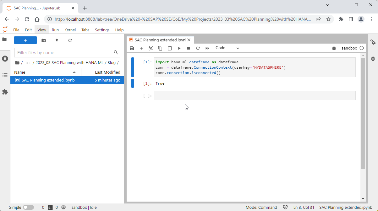
To start working with the data, create a hana_ml Dataframe, that points to the view, that accesses the user input. This is the view, which was created in the previous blog (ie "ExtSACP01_FactData_View"). To improve calculation performance save the data into a temporary table in SAP Datasphere, here called "#PLANNINGDATA". All data is staying in the cloud. Just display a few rows to verify that the data is available.
df_remote = conn.table('ExtSACP01_FactData_View', schema='EXTEND_SAC_PLANNING')

df_remote = df_remote.save('#PLANNINGDATA', table_type='LOCAL TEMPORARY', force=True)

df_remote.head(10).collect()
First we train a simple Machine Learning model on the actuals data, to use the UnitPrice as Predictor to explain the UnitsSold. This requires some semantical data transformation. In the original structure these two values that belong to the same months (UnitPrice and UnitsSold) are spread across two rows of data. Structure the data, so that both values for the same month become columns for the same row. Display a few rows to verify the output.
df_remote_act = df_remote.filter(""" "Version" = 'public.Actual'""")

df_remote_act = df_remote_act.filter('''"Account" = 'UnitPrice' ''').rename_columns({'Value': 'UnitPrice'}).select('Date', 'UnitPrice').set_index('Date').join(

    df_remote_act.filter('''"Account" = 'UnitsSold' ''').rename_columns({'Value': 'UnitsSold'}).select('Date', 'UnitsSold').set_index('Date'), how='left'

)

df_remote_act.head(5).collect()
Similarly, prepare the data on which the model will be applied to estimate future sales quantities. We use the planned UnitPrice for the months, for which no actuals are available yet (April to December 2023 in this example).
df_remote_plan = df_remote.filter(""" "Version" = 'public.Plan'""")

df_remote_plan = df_remote_plan.filter('''"Account" = 'UnitPrice' ''').rename_columns({'Value': 'UnitPrice'}).select('Date', 'UnitPrice').set_index('Date').join(

    df_remote_plan.filter('''"Account" = 'UnitsSold' ''').rename_columns({'Value': 'UnitsSold'}).select('Date', 'UnitsSold').set_index('Date'), how='left'

)

month_last_actual = df_remote_act.select('Date').max()

df_remote_plan = df_remote_plan.filter(f'''"Date" > '{month_last_actual}' ''')

df_remote_plan.head(10).collect()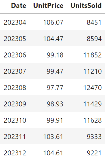
Trigger the training of the Machine Learning model, using the embedded Machine Learning in SAP Datasphere. We use a simple linear regression.
from hana_ml.algorithms.pal.unified_regression import UnifiedRegression

ur_hgbt = UnifiedRegression(func='LinearRegression')

ur_hgbt.fit(data=df_remote_act, features=['UnitPrice'], label='UnitsSold')
We are not testing the model further. Let's just have a quick look at the model quality. An R'2 of 0.96 shows that the model describes the relationship between UnitPrice and UnitsSold extremely well. We are using sample data. Should your own models on real data come with similar statistics, you may want to be suspicious that something went wrong.
from hana_ml.visualizers.unified_report import UnifiedReport

UnifiedReport(ur_hgbt).build().display()
Now apply the trained model to predict the UnitsSold for the future months, based on the planned UnitPrice for each month. The prediction itself is just one line of code. The remainder of the code structures the data to be in the necessary format so that SAC Planning can import it later on.
df_rem_predicted = ur_hgbt.predict(data=df_remote_plan, features='UnitPrice', key='Date')

df_rem_predicted = df_rem_predicted.drop(['LOWER_BOUND', 'UPPER_BOUND', 'REASON'])

df_rem_predicted = df_rem_predicted.rename_columns({'SCORE': 'Value'})

df_rem_predicted = df_rem_predicted.add_constant('Version', 'public.Plan')

df_rem_predicted = df_rem_predicted.add_constant('Category', 'Planning')

df_rem_predicted = df_rem_predicted.add_constant('Account', 'UnitsSold')

df_rem_predicted = df_rem_predicted.select('Version', 'Date', 'Account', 'Value', 'Category')

df_rem_predicted.head(5).collect()
And save those predictions to a physical table in SAP Datasphere, from where SAC Planning can import the data.
df_rem_predicted.save('CUSTOM_CALCULATIONS', force=True)You can now see the forecasts in the table, for example via the SAP HANA Database Explorer or in tools like DBeaver.
Deploying the calculation code
Once we are happy with the code from the Jupyter Notebook, it needs to be callable via REST-API, to be integrated into the SAC Planning workflow. For the deployment of that Python code you can use any environment that is able to expose such code as REST-API, for instance Cloud Foundry, Kyma or SAP Data Intelligence.
In this example we use Cloud Foundry, which is a very lightweight deployment on the SAP Business Technology Platform. In case you haven't deployed Python code yet on Cloud Foundry, you can familiarise yourself with the blog Scheduling Python code on Cloud Foundry. In our case however, we don't need to schedule any code, hence you can ignore that part of the blog. You do not need to create instances of the "Job Scheduler" and "Authorization & Trust Management (XSUAA)" services.
For creating the REST-API that is to be called from SAC Planning four files are required. All necessary code is listed in this blog, but remember that you can also download the actual files from the samples repository.
File 1 of 4: sacplanningmlunitssold.py
This file contains the code that gets executed when the REST-API is called. It is mostly the code that was created in the Jupyter Notebook. Personally, I am creating such a Python file in Visual Studio Code, but any Python environment should be fine.
Hint: The REST-API needs to have both a GET and POST endpoint. The GET endpoint is required so that SAP Analytics Cloud can save a connection for that endpoint. The POST endpoint is required by the multi-action, that operationalises the code.
from flask import Flask

from flask import Response

import os, json, IPython

from hana_ml import dataframe

from hana_ml.algorithms.pal.unified_regression import UnifiedRegression


app = Flask(__name__)

# Port number is required to fetch from env variable

# http://docs.cloudfoundry.org/devguide/deploy-apps/environment-variable.html#PORT


cf_port = os.getenv("PORT")


# Get SAP HANA logon credentials from user-provided variable in CloudFoundry

hana_credentials_env = os.getenv('HANACRED')

hana_credentials = json.loads(hana_credentials_env)

hana_address = hana_credentials['address']

hana_port = hana_credentials['port']

hana_user = hana_credentials['user']

hana_password = hana_credentials['password']


# POST method as required by SAC PLanning

@app.route('/', methods=['GET', 'POST'])

def processing():


	# Connect to SAP HANA Cloud

	conn = dataframe.ConnectionContext(address=hana_address,

                                   port=hana_port,

                                   user=hana_user,

                                   password=hana_password)


	# Move planning data to staging table (for performance)

	df_remote = conn.table('ExtSACP01_FactData_View', schema='EXTEND_SAC_PLANNING')

	df_remote = df_remote.save('#PLANNINGDATA', table_type='LOCAL TEMPORARY', force=True)


	# Prepare the actuals data to train the model

	df_remote_act = df_remote.filter(""" "Version" = 'public.Actual'""")

	df_remote_act = df_remote_act.filter('''"Account" = 'UnitPrice' ''').rename_columns({'Value': 'UnitPrice'}).select('Date', 'UnitPrice').set_index('Date').join(

    df_remote_act.filter('''"Account" = 'UnitsSold' ''').rename_columns({'Value': 'UnitsSold'}).select('Date', 'UnitsSold').set_index('Date'), how='left'

)

	# Prepare the planning data to predict the future (months without actuals)

	df_remote_plan = df_remote.filter(""" "Version" = 'public.Plan'""")

	df_remote_plan = df_remote_plan.filter('''"Account" = 'UnitPrice' ''').rename_columns({'Value': 'UnitPrice'}).select('Date', 'UnitPrice').set_index('Date').join(

		df_remote_plan.filter('''"Account" = 'UnitsSold' ''').rename_columns({'Value': 'UnitsSold'}).select('Date', 'UnitsSold').set_index('Date'), how='left'

	)

	month_last_actual = df_remote_act.select('Date').max()

	df_remote_plan = df_remote_plan.filter(f'''"Date" > '{month_last_actual}' ''')


	# Train and apply the Machine Learning model

	ur_hgbt = UnifiedRegression(func='LinearRegression')

	ur_hgbt.fit(data=df_remote_act, features=['UnitPrice'], label='UnitsSold')

	df_rem_predicted = ur_hgbt.predict(data=df_remote_plan, features='UnitPrice', key='Date')


	# Prepare dataset for returning to SAC Planning

	df_rem_predicted = df_rem_predicted.drop(['LOWER_BOUND', 'UPPER_BOUND', 'REASON'])

	df_rem_predicted = df_rem_predicted.rename_columns({'SCORE': 'Value'})

	df_rem_predicted = df_rem_predicted.add_constant('Version', 'public.Plan')

	df_rem_predicted = df_rem_predicted.add_constant('Category', 'Planning')

	df_rem_predicted = df_rem_predicted.add_constant('Account', 'UnitsSold')

	df_rem_predicted = df_rem_predicted.select('Version', 'Date', 'Account', 'Value', 'Category')


	# Save the data into staging table

	df_rem_predicted.save('CUSTOM_CALCULATIONS', force=True)


	# Process compelete

	return Response("{'message':'The data has been processed'}", status=200, mimetype='application/json')


if __name__ == '__main__':

	if cf_port is None:

		app.run(host='0.0.0.0', port=5000, debug=True)

	else:

		app.run(host='0.0.0.0', port=int(cf_port), debug=True)
File 2 of 4: manifest.yml
The manifest specifies for instance the memory requirements for the application.
---

applications:

- memory: 128MB

  command: python sacplanningmlunitssold.py

  random-route: true
File 3 of 4: runtime.txt
The runtime file specifies the Python version that is to be used.
python-3.9.xFile 4 of 4: requirements.txt
The requirements file specifies the Python libraries that are to be installed.
Flask

hana-ml==2.15.23011100

shapely

IPython
Place these four files into a local folder on your laptop. Now push them to Cloud Foundry as application. This concept was introduced in the blog mentioned above, Scheduling Python code on Cloud Foundry. Since the application requires the database credentials, which haven't been provided yet, the application is pushed, but not started yet.
cf7 push sacplanningmlunitssold --no-startNow store the database credentials in a user-defined variable in Cloud Foundry, from where the application can retrieve them.
cf7 set-env sacplanningmlunitssold HANACRED {\"address\":\"REPLACEWITHYOURHANASERVER\",\"port\":443,\"user\":\"REPLACEWITHYOURUSER\",\"password\":\"REPLACEWITHYOURPASSWORD\"}Everything is in place. Start the Cloud Foundry application and the path of the REST-API is displayed.
cf7 start sacplanningmlunitssold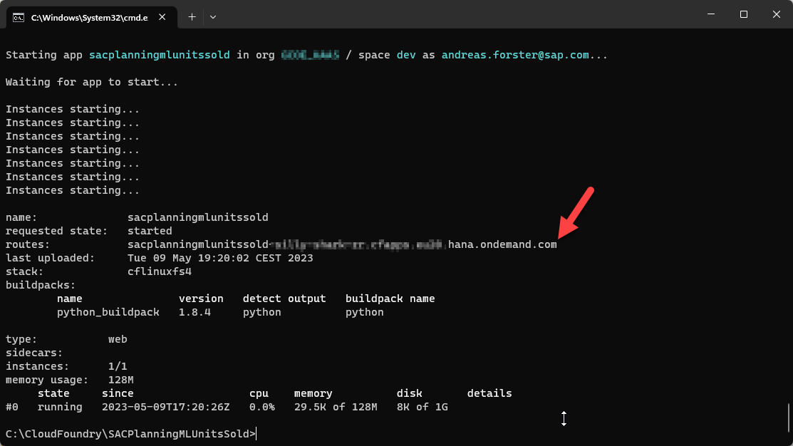
Calling this REST-API triggers the logic in the sacplanningcustomcalc.py file. The code connect to the SAP HANA Cloud system that is part of SAP Datasphere. It instructs SAP HANA Cloud to work with the SAC Planning values. A Machine Learning model is trained on the actuals data to explain the UnitsSold based on the UnitsPrice. For future months the planned UnitsPrice is used to predict the estimated UnitsSold. . That forecast is written to the staging table, where SAC Planning can pick then up.
Before embedding the REST-API into the workflow, just give it a test. You can use Postman for instance. Call the POST endpoint, which should result in the staging table being updated.

The REST-API is up and running. Calling it triggers the Machine Learning forecasts, which are written to the staging table. We conclude the blog by showing how to make this REST-API accessible to SAP Analytics Cloud.
SAP Analytics Cloud can access REST-APIs that support "Basic Authentication" or "OAuth 2.0 Client Credentials". In our example we take the OAuth option. Hence "Add a New OAuth Client" in SAP Analytics Cloud → Administration → App Integration. We name the client here "CloudFoundry for Custom ML". Keep the default settings, just enter the path of the REST-API into the "Redirect URI" option. Be sure to add "https://" in front.

When the client has been created, note down the following values. They will be needed in the next step.
- OAuth Client ID
- Secret:
- Token URL
Still in SAP Analytics Cloud, create now a new connection of type "HTTP API".

Enter these values:
- Connection Name: API CloudFoundry for Custom ML
- Data Service URL: [The same URL as used in the previous step as "Redirect URI"]
- Authentication Type: OAuth 2.0 Client Credentials
- OAuth Client ID: [The ID you received in the previous step]
- Secret: [The secret you received in the previous step]
- Token URL: [also from the previous step]
The connection has been created. SAP Analytics Cloud can now call the REST-API to trigger the Machine Learning.
![]()
Summary / What's next
In the steps described in this blog we accessed the planning data from the SAC Planning model to create predictions, which are written into a temporary staging table.
In the next blog you will see how this data can be imported into the planning model and how the whole process can be operationalised.
Bonus section
Early on in the above coding example it was mentioned, that you can keep your database password safe in the Secure User Store. Here are the steps to set this up:
Step 1: Install on the machine, on which you execute the notebook (probably your laptop), the SAP HANA Client 2.0. This also installs the Secure User Store.
Step 2: Save your database credentials in the Secure User Store. Open your operating system's command prompt (ie cmd.exe on Windows). Navigate in that prompt to the SAP HANA Client's installation folder (ie 'C:\Program Files\SAP\hdbclient'. The following command stores the credentials under the key MYDATASPHERE. You can change the name of the key as you like.
hdbuserstore -i SET MYDATASPHERE "[YOURENDPOINT]:443" [YOURDBUSER]Step 3: Now the hana_ml package can pull the credentials from the Secure User Store to establish a connection. The code does not contain the password in clear text anymore.
import hana_ml.dataframe as dataframe

conn = dataframe.ConnectionContext(userkey='MYDATASPHERE')

conn.connection.isconnected()
Labels:
3 Comments
You must be a registered user to add a comment. If you've already registered, sign in. Otherwise, register and sign in.
Labels in this area
-
ABAP CDS Views - CDC (Change Data Capture)
2 -
AI
1 -
Analyze Workload Data
1 -
BTP
1 -
Business and IT Integration
2 -
Business application stu
1 -
Business Technology Platform
1 -
Business Trends
1,658 -
Business Trends
93 -
CAP
1 -
cf
1 -
Cloud Foundry
1 -
Confluent
1 -
Customer COE Basics and Fundamentals
1 -
Customer COE Latest and Greatest
3 -
Customer Data Browser app
1 -
Data Analysis Tool
1 -
data migration
1 -
data transfer
1 -
Datasphere
2 -
Event Information
1,400 -
Event Information
67 -
Expert
1 -
Expert Insights
177 -
Expert Insights
301 -
General
1 -
Google cloud
1 -
Google Next'24
1 -
GraphQL
1 -
Kafka
1 -
Life at SAP
780 -
Life at SAP
13 -
Migrate your Data App
1 -
MTA
1 -
Network Performance Analysis
1 -
NodeJS
1 -
PDF
1 -
POC
1 -
Product Updates
4,577 -
Product Updates
346 -
Replication Flow
1 -
REST API
1 -
RisewithSAP
1 -
SAP BTP
1 -
SAP BTP Cloud Foundry
1 -
SAP Cloud ALM
1 -
SAP Cloud Application Programming Model
1 -
SAP Datasphere
2 -
SAP S4HANA Cloud
1 -
SAP S4HANA Migration Cockpit
1 -
Technology Updates
6,873 -
Technology Updates
429 -
Workload Fluctuations
1
Related Content
- WebIDE: Extending Create Purchase Requisition New (F1643A) in Technology Q&A
- Enhanced Data Analysis of Fitness Data using HANA Vector Engine, Datasphere and SAP Analytics Cloud in Technology Blogs by SAP
- SAP Sustainability Footprint Management: Q1-24 Updates & Highlights in Technology Blogs by SAP
- Custom data as table, CDS, Domain, Business object and all that jazz... in Technology Blogs by SAP
- SAP Datasphere - Space, Data Integration, and Data Modeling Best Practices in Technology Blogs by SAP
Top kudoed authors
| User | Count |
|---|---|
| 34 | |
| 17 | |
| 15 | |
| 14 | |
| 11 | |
| 9 | |
| 8 | |
| 8 | |
| 8 | |
| 7 |