
- SAP Community
- Products and Technology
- Technology
- Technology Blogs by SAP
- HANA based Transformation (deep dive)
Technology Blogs by SAP
Learn how to extend and personalize SAP applications. Follow the SAP technology blog for insights into SAP BTP, ABAP, SAP Analytics Cloud, SAP HANA, and more.
Turn on suggestions
Auto-suggest helps you quickly narrow down your search results by suggesting possible matches as you type.
Showing results for
Advisor
Options
- Subscribe to RSS Feed
- Mark as New
- Mark as Read
- Bookmark
- Subscribe
- Printer Friendly Page
- Report Inappropriate Content
06-17-2016
9:42 PM
2 HANA based Transformation (deep dive)
This blog is part of the blog series HANA based BW Transformation.
Now I will look a little bit behind the curtain and provide some technical background details about SAP HANA Transformations. The information provided here serves only for a better understanding of BW transformations which are pushed down.
As part of the analysis of HANA executed BW transformations we need to distinguish between simple (non-stacked) and stacked data flows. A simple, non-stacked data flow connects two persistent objects with no InfoSource in between, only one BW transformation is involved. We use the term stacked data flow for a data flow with more than one BW transformation and at least one InfoSource in between.
| Stability of the generated runtime objects |
|---|
All information I provide here are background information to get a better understanding on SAP HANA executed BW transformation. It is important to keep in mind that all object definition could be changed! Do not implement any stuff based on the generated objects! The
|
2.1 Simple data flow (Non-Stacked Data Flow)
A simple data flow is a data flow which connects two persistent BW objects with no InfoSource in between. The corresponding Data Transfer Process (DTP) processes only one BW transformation.
In case of a non-stacked data flow the DTP reuses the SAP HANA Transformation (SAP HANA Analysis Process) of the BW transformation, see Figure 2.1.

Figure 2.1: Non-Stacked Transformation
2.2 Stacked Data Flow
A stacked data flow connects two persistent data objects with at least one InfoSource in between. Therefore a stacked data flow contains at least two BW transformations. The corresponding Data Transfer Process (DTP) processes all involved BW transformations.
In case of a stacked data flow, the DTP cannot use the SAP HANA Transformation (SAP HANA Analysis Process) of the BW transformations. Strictly speaking, it is not possible to create a CalcScenario for a BW transformation with an InfoSource as source object. An InfoSource cannot be used as a data source in a CalculationScenario.

Figure 2.2: Stacked Transformation
Figure 2.2 shows a stacked data flow with two BW transformations (1) and (2) and the corresponding SAP HANA Transformations (3) and (4). There is no tab for the CalculationScenario in the SAP HANA Transformation (3) for the BW transformation (1) with an InfoSource as source object.
Therefore the DTP generated its own SAP HANA Transformations (6) and (7) for each BW transformation. The SAP HANA Transformations for the DTP are largely equivalent to the SAP HANA Transformation for the BW transformations (3) and (4).
In the sample data flow above, the SAP HANA Transformation (5) for the DTP get its own technical ID TR_5I3Y6060H25LXFS0O67VSCIF8. The technical ID is based on the technical DTP ID and the prefix DTP_ would be replaced by the prefix TR_.
The SAP HANA Transformation (5) and (6) is only a single object, in fact. I included it twice in the picture to illustrate that the SAP HANA Transformation (6) is based on the definition of the BW transformation (1) and will be used (5) from the DTP.
Figure 2.3 provides a more detailed view of the generated SAP HANA Transformation. The SAP HANA Transformation (6) is based on the definition of the BW transformation (1) and is therefore largely identical to the SAP HANA Transformation (3). (3) and (6) differs only in the source object. The SAP HANA transformation (6) uses the SAP HANA Transformation / SAP HANA Analysis Process (7) as the source object instead of the InfoSource as shown in (3). The SAP HANA Transformations (4) and (7) are also quite similar. They only differ with respect to the target object. In the SAP HANA Transformation (3), the InfoSource is used as the target object. The SAP HANA transformation (7) does not have an explicit target object. Its target object is only marked as Embedded in a Data Transfer Process. That means the SAP HANA Transformation (7) is used as data source in a SAP HANA Transformation, in our case in the SAP HANA Transformation (6).
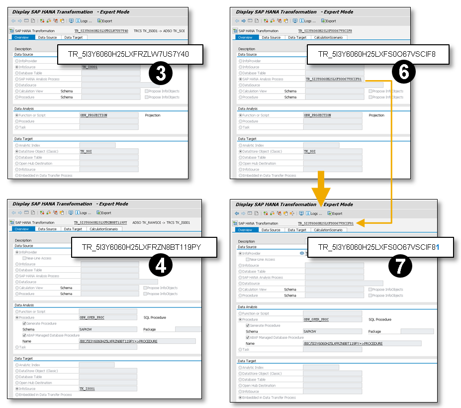
Figure 2.3: Stacked Transformation (detailed)
The technical ID of the embedded SAP HANA Transformation (7) is based on the technical ID of the SAP HANA Transformation (5) and (6) of the DTP. Only the last digit 1 will be added as a counter for the level. This means that in case of a stacked data flow with more than two BW transformations, the next SAP HANA Transformation would get the additional digit 2 instead of 1 and so on.
Later on we will need the technical IDs to analyze a HANA based BW transformation, therefore it is helpful to understand how they are being created.
2.3 CalculationScenario
To analyze a SAP HANA based BW transformation, it is necessary to understand the primary SAP HANA runtime object, the CalculationScenario (CalcScenario). The BW Workbench shows the CalcScenario in an XML representation, see (2) in Figure 2.4. The CalculationScenario is part of the corresponding SAP HANA Transformation (Extra è Generated Program HANA Transformation) of the DTP. The CalculationScenario tab is only visible if the Expert Mode (Extras è Expert Mode on/off) is switched on. Keep in mind, if the source object of the BW transformation is an InfoSource the CalculationScenario could only been reached by using the DTP Meta data, see »Dataflow with more than one BW transformation« and »Stacked Data Flow«.
The naming convention for the CalculationScenario is:
/1BCAMDP/0BW:DAP:<Technical ID – SAP HANA Transformation>
The CalculationScenario shown in the CalculationScenario tab, see (2) and (1) in Figure 2.4, is only a local temporary version, therefore the additional postfix .TMP.
The CalculationScenario processes the transformation logic by using different views (CalculationViews) to split the complex logic into more simplified single steps. One CalculationView, the default CalculationView, represents the CalculationScenario itself. The default CalculationView uses one or more other CalculationViews as source and so on, see Figure 2.5. A CalculationView cannot be used in SQL statements, therefore for each CalculationView a ColumnView will be generated.
Inside the SAP HANA database, the ColumnViews are created in the SAP<SID> schema, see (1). Each ColumnView represents a CalculationView, see paragraph 2.3.2.1 »CalculationScenario - calculationViews«, within a CalculationScenario. The create statement of each ColumnView provides two objects. First the CalculationScenario and as second object the ColumnView based on the CalculationScenario. All ColumnViews that belong to a SAP HANA transformation are based on the same CalculationScenario.

Figure 2.4: CalculationScenario and ColumnViews
SAP HANA internally uses the JSON notation to represent a CalculationScenario. Figure 2.5 shows the CalculationScenario depicted in Figure 2.4 (2) in a JSON Analyzer. The tree representation provides a good overview how the different CalculationViews are consumed. The JSON based CalcScenario definition can be found in the Create Statement tab in the column view definition in the SAP HANA studio. The definition can be found in the USING clause of the CREATE CALCULATION SCENARIO statement, the definition starts with ‘[‘ and ends with ‘]’.

Figure 2.5: CalculationScenario in a JSON Analyzer
The SAP HANA studio also provides a good tool to visualize a CalculationScenario, see Figure 2.6. To open the visualization tool click on Visualize View in the context menu of a ColumnView based on a CalculationScenario. The visualization view is divided in three parts. The first part (1) provides a list of the CalculationViews which are used inside the CalculationScenario. Depending on each view definition there are more information about variables, filter or attributes are below the view node available. The second part (2) provides an overview about the view dependencies. Which view consumes which view? The third part (3) provides context sensitive information for a view form the second part.

Figure 2.6: CalculationScenario visualization in the SAP HANA Studio
Now we will have a deeper look into the following sub nodes of the calculationScenario node (see (2) in Figure 2.4):
- dataSources
- variables
- calculationViews
2.3.1 CalculationScenario - dataSources
The node dataSources lists all available data source objects of the CalculationScenario. The following data sources are used within a CalculationScenario in the context of a BW transformation:
- tableDataSource
- olapDataSource
- calcScenarioDataSource
In the first sample transformation, we only use a database table (tableDataSource) as the source object, see Figure 2.7. The sample data flow reads from a DataSource (RSDS), therefore the corresponding PSA table is defined as tableDataSource. To resolve the request ID, the SID table /BI0/SREQUID is also added to the list of data sources.

Figure 2.7: CalculationScenario – Node: TableDataSource
In the second sample a transformation rule Master data read is being used in the BW transformation. In this case an olapDataSource is added to the list of data sources. The olapDataSourceuses the logical index (0BW:BIA:0MATERIAL_F4) from the InfoObject to read the required master data from the real source tables, see Figure 2.8.
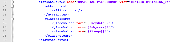
Figure 2.8: CalculationScenario – Node: OLAPDataSource
To read the master data in the requested language, object version and time the PLACEHOLDERS
- keydate,
- objvers
- langu
are added.
The third sample is a stacked data flow. In a stacked data flow the CalculationScenario from the DTP uses another CalculationScenario as data source. In these cases, the calcScenarioDataSource is used. The variables defined in the upper CalculationScenario are passed to the underlying CalculationScenario to be able to push down these variables (filters) where possible to the source objects, see Figure 2.9.

Figure 2.9: CalculationScenario – Node: CalcScenarioDataSource
The values for the PLACEHOLDERS are passed in the SQL statement by using the variables, see paragraph 2.3.2 »CalculationScenario - variables«.
The variables for the PLACEHOLDER for the variables keydate, objvers and langu are always set in the INSERT AS SELECT statement, whether they are used or not.
2.3.2 CalculationScenario - variables
In the node variables, all parameters are defined which are used in the CalculationScenario and can be used in the SQL statement to filter the result, see Figure 2.10.

Figure 2.10: CalculationScenario – Node: variables
| Placeholder usage by customer |
|---|
All variables and placeholders defined in a CalculationScenario in the context of a BW transformation are only intended for SAP internal usage. Variables and placeholder names are not stable, that means they can be changed, replaced or removed. |
Figure 2.11 provides a further sample, based on a BW transformation, with several dataSource definitions. A variable is been used to control which dataSource and at the end from which table the data are read by the SQL statement.
The sample data flow for this CalculationScenario reads from an advanced DSO (ADSO) (based on a Data Propagation Layer - Template) with three possible source tables (Inbound Table, Change Log and Active Data). For each source table (dataSource), at least one view is generated into the CalculationScenario and all three views are combined by a union operation, see (2).
The input nodes are used to enhance all three structures by a new constant field named BW_HAP__________ADSO_TABLE_TYPE. The constant values
- Inbound Table (AQ),
- Change Log (CL) and
- Active Data (AT)
can later be used as values for the filter $$ADSO_TABLE_TYPE$$, see (3). The filter value is handed over by the SELECT statement and depends, for example, on the DTP settings (Read from Active Table or Read from Change Log). To read data only from the active data (AT) table the following placeholder setting is used:
'PLACEHOLDER'=('$$adso_table_type$$', '( ("BW_HAP__________ADSO_TABLE_TYPE"=''AT'' ) )'),
For further information see 2.4 »SQL Statement«.

Figure 2.11: CalculationScenario – DataSource and Variable collaboration
2.3.2.1 CalculationScenario - calculationViews
The next relevant node type is the node calculationView. A CalculationScenario uses several layered views (calculationView) to transfer the logic given by the BW transformation. For the CalculationScenario and for each calculationView, a ColumnView is created, see (1) in Figure 2.4. The CalculationScenario related to a column view can be found in the definition of each column view.
There are several view types which can be used as sub node of a calculationView:
- projection
- union
- join
- aggregation
- unitConversion
- verticalUnion
- rownum
- functionCall
- datatypeConversion
- …
The view types as well as the number of views used in a CalculationScenario depend on the logic defined in the BW transformation and the BW / SAP HANA release.
A SELECT on a CalculationScenario (ColumnView) always reads from the default view. There is only one default view allowed. The default view can been identified by checking whether the attribute defaultViewFlag is set to “true”. In the JSON representation in Figure 2.5, the default view is always shown as the top node.
The processing logic of each view is described in further sub nodes. The most important sub nodes are:
- viewAttributesattributes
- inputs
- filter
The used sub nodes of a CalculationView depend on the view type, on the logic defined in the BW transformation, and the BW / SAP HANA release.
CalculationScenario - calculationViews – view - viewAttributes / attributes
The nodes viewAttributes and attributes are used to define the target structure of a calculation view. The node attributes is used for more complex field definitions like data type mapping and calculated attributes (calculatedAttributes ).
The InfoObject TK_MAT is defined as CHAR(18) with a conversion routine ALPHA. To ensure that all values comply with the APLHA conversion rules, the CalculationScenario creates an additional field TK_MAT$TMP as a calculatedAttribute. Figure 2.12 shows the definition of the new field. The APLHA conversion rule logic is implemented as a formula based on the original field TK_MAT.

Figure 2.12: CalculationScenario - CalculationAttributes
Calculated attributes are memory-intensive and we try to avoid them where possible. But there are some scenarios where calculated attributes must be used. For example, in case of target fields based on InfoObjects with conversion routines (see Figure 2.12) and in case of “non-trustworthy” sources. A “non-trustworthy” data source is a field-based source object (that is not based on InfoObjects), for example a DataSource (RSDS) or a field based advanced DataStore-Object (ADSO). In case of “non-trustworthy” data sources, the CalculationScenario must ensure that NULL values are converted to the correct type-related initial values.
CalculationScenario - calculationViews – view – inputs
A calculation view can read data from one or more sources (inputs). CalculationViews and/or data sources could be used as sources. They are listed under the node input. A projection or an aggregation, for example, typically have one input node, and a union or a join typically have more than one input node.
The input node in combination with the mapping and viewAttribute nodes can be used to define new columns. In Figure 2.13 the attribute #SOURCE#.1.0REQTSN is defined as a new field based on the source field 0REQTSN.

Figure 2.13: CalculationScenario - input
CalculationScenario - calculationViews – view – filter
The filter node, see (2) in Figure 2.14, is used in combination with the variable, see (1) in Figure 2.14, to provide the option to filter the result set of the union-view (TK_SOI). The filter value is set as placeholder in the SQL statement see (3) in Figure 2.14

Figure 2.14: CalculationScenario - input
I will come back to the different views later on in the analyzing and debugging section.
2.4 SQL Statement
Running a DTP triggers an INSERT AS SELECT statement that reads data from the source and directly inserts the transformed data into the target object. There are two kinds of filter options available to reduce the processed data volume: the WHERE condition in the SQL statement and the Calculation Engine PLACEHOLDER. Placeholders are used to set values for variables / filters which are defined in the CalculationScenario. Which placeholders are used depends on the logic defined in the BW transformation and the BW / SAP HANA release.
PLACEHOLDER
The following table describes the most important PLACEHOLDERS which can be embedded in a CalculationScenario and used in the SQL statements. Which PLACEHOLDERis been used in the CalculationScenario depends on the implemented dataflow logic.
| Important note about the PLACEHOLDER |
|---|
PLACEHOLDER are not stable and the definition can be changed by a new release, support package or note! It is not supported to use the here listed PLACEHOLDER inside a SQL Script or any other embedded database object in a context of a BW transformation. This also applies to all PLACEHOLDER used in the generated SQL statement. |
Placeholder name | Description |
$$client$$ | Client value to read client dependent data. The placeholder is always set, whether it is used or not. |
$$change_log_filter$$ | This placeholder is only used to filter the data which is read from the change log. The filter values are equivalent to the values of the placeholder $$filter$$. The placeholder is only used for advanced DataStore-Objects (ADSO). See also $$inbound_filter$$ and $$nls_filter$$. |
$$change_log_extraction$$ | Wenn die Extraktion aus dem Changelog erfolgt ist der Wert ‘X’ gesetzt. Wird im Rahmen des Errorhandlings genutzt. |
$$datasource_src_type$$ | The placeholder is set to ‚X‘ in case the data would be read from the remote source object and not from the PSA. |
$$dso_table_type$$ | This placeholder is used to control which table of a standard DataStore-Object (ODSO) is used as data source. Therefore the field BW_HAP__________DSO_TABLE_TYPE can be set to:
|
$$filter$$ | This placeholder is used to filter the source data where possible. That means the placeholder is typically used in the next view above the union for all available source tables. This placeholder contains the filters defined in the DTP extraction tab plus some technical filters based on the REQUEST or the DATAPAKID. In case of using an ABAP routine or a BEx-Variable in the DTP filter, the result of both are used to create the filter condition. The placeholder $$filter$$ is used for all BW objects except advanced DataStore-Objects (ADSO). To filter an ADSO see $$inbound_filter$$, $$change_log_filter$$ and $$nls_filter$$. |
$$inbound_filter$$ | This placeholder is only used to filter the data which is read from the inbound queue[KT1] . The filter values are equivalent to the values of the placeholder $$filter$$. This placeholder is only used for advanced DataStore-Objects (ADSO). See also $$change_log_filter$$ and $$nls_filter$$. |
$$changelog_filter$$ | This placeholder is only used to filter the data which is read from the change log. The filter values are equivalent to the values of the placeholder $$filter$$. This placeholder is only used for advanced DataStore-Objects (ADSO). See also $$change_log_filter$$ and $$nls_filter$$. |
$$keydate$$ | Date to read time dependent master data. The variable value is applied to the logical index of an InfoObject in an olapDataSource. The variable is always set, whether it is used or not. |
$$langu$$ | Language to read master data. The variable value is applied to the logical index of an InfoObject in an olapDataSource. The placeholder is always set, whether it is used or not. |
$$navigational_attribute_filter$$ | This placeholder lists the filters based on navigation attributes, which are used in the DTP filter. |
$$objvers$$ | Object version to read master data. The variable value is applied to the logical index of an InfoObject in an olapDataSource. The variable is always set, whether it is used or not. |
$$runid$$ | For some features, it is necessary to store metadata in a temporary table. In a prepare phase, the metadata is inserted into this temporary table identified by a unique id (runid). During runtime, the values are then read by using the runid of this placeholder. This placeholder is primarily used in a CalcScenario based on an explicitly created SAP HANA Analysis Process (see transaction RSDHAAP) and not a SAP HANA Transformation. |
$$target_filter$$ | The target filter is used in a SQL statement to ensure that only those records of the result set which match this filter condition are inserted into a target object. This placeholder is used if the filter condition is given by the target object, for example by a semantically partitioned Object (SPO). A target filter is applied to the result set of the transformation. |
$$datasource_psa_version$$ | Relevant version number of the PSA where the current request is located. |
$$DATAPAKID$$.DTP | This value is set by the package size parameter maintained in the DTP. More information, especially for dependencies, can be found in the value help (F1) for the DTP package size parameter. |
$$REQUEST$$.DTP | This placeholder contains the request ID for the target request. In the simulation mode, the value is always set to the SID value of the request ID DTPR_SIMULATION in the request table /BI0/SREQUID. |
The following SQL SELECT statement, see Figure 2.15, belongs to the CalculationScenario as shown in Figure 2.11. The SQL statement passes the value for the variable adso_table_type. The placeholder
'PLACEHOLDER'=('$$adso_table_type$$', '( ("BW_HAP__________ADSO_TABLE_TYPE"=''AT'' ) )'),
sets the field BW_HAP__________ADSO_TABLE_TYPE to ’AT’. In the union definition in Figure 2.11, see (2), the field BW_HAP__________ADSO_TABLE_TYPE is set to the constant value ’AT’ for all rows provided by the active data table. Like this, the placeholder ensures that only data from the active data table is selected.

Figure 2.15: DPT - SELECT statement
Some PLACEHOLDERS get the transformation-ID as a prefix to ensure that these PLACEHOLDER identifiers are unique, see placeholder $$runid$$ in Figure 2.15 and the calcScenarioDataSource description in the blog HANA based BW Transformation
- SAP Managed Tags:
- BW (SAP Business Warehouse)
8 Comments
You must be a registered user to add a comment. If you've already registered, sign in. Otherwise, register and sign in.
Labels in this area
-
ABAP CDS Views - CDC (Change Data Capture)
2 -
AI
1 -
Analyze Workload Data
1 -
BTP
1 -
Business and IT Integration
2 -
Business application stu
1 -
Business Technology Platform
1 -
Business Trends
1,658 -
Business Trends
107 -
CAP
1 -
cf
1 -
Cloud Foundry
1 -
Confluent
1 -
Customer COE Basics and Fundamentals
1 -
Customer COE Latest and Greatest
3 -
Customer Data Browser app
1 -
Data Analysis Tool
1 -
data migration
1 -
data transfer
1 -
Datasphere
2 -
Event Information
1,400 -
Event Information
72 -
Expert
1 -
Expert Insights
177 -
Expert Insights
340 -
General
1 -
Google cloud
1 -
Google Next'24
1 -
GraphQL
1 -
Kafka
1 -
Life at SAP
780 -
Life at SAP
14 -
Migrate your Data App
1 -
MTA
1 -
Network Performance Analysis
1 -
NodeJS
1 -
PDF
1 -
POC
1 -
Product Updates
4,575 -
Product Updates
384 -
Replication Flow
1 -
REST API
1 -
RisewithSAP
1 -
SAP BTP
1 -
SAP BTP Cloud Foundry
1 -
SAP Cloud ALM
1 -
SAP Cloud Application Programming Model
1 -
SAP Datasphere
2 -
SAP S4HANA Cloud
1 -
SAP S4HANA Migration Cockpit
1 -
Technology Updates
6,872 -
Technology Updates
472 -
Workload Fluctuations
1
Related Content
- Inside SAP: Discover How SAP’s IT Drives Transformation and Innovation in Technology Blogs by SAP
- Be a Cockroach: A Simple Guide to AI and SAP Full-Stack Development - Part I in Technology Blogs by Members
- Tracking HANA Machine Learning experiments with MLflow: A conceptual guide for MLOps in Technology Blogs by SAP
- Syniti RDG provides an effortless way to create Data Model extension. in Technology Q&A
- Tracking HANA Machine Learning experiments with MLflow: A technical Deep Dive in Technology Blogs by SAP
Top kudoed authors
| User | Count |
|---|---|
| 17 | |
| 14 | |
| 12 | |
| 10 | |
| 9 | |
| 8 | |
| 7 | |
| 7 | |
| 6 | |
| 6 |