


- SAP Community
- Products and Technology
- Enterprise Resource Planning
- ERP Blogs by SAP
- Part 3: SAP S/4HANA Migration Cockpit - Using SA...
Enterprise Resource Planning Blogs by SAP
Get insights and updates about cloud ERP and RISE with SAP, SAP S/4HANA and SAP S/4HANA Cloud, and more enterprise management capabilities with SAP blog posts.
Turn on suggestions
Auto-suggest helps you quickly narrow down your search results by suggesting possible matches as you type.
Showing results for
Product and Topic Expert
Options
- Subscribe to RSS Feed
- Mark as New
- Mark as Read
- Bookmark
- Subscribe
- Printer Friendly Page
- Report Inappropriate Content
12-02-2019
9:43 AM
This is the third part of a blog series on how to load data to the staging tables of the SAP S/4HANA migration cockpit. This part explains how to load data to the staging tables using the HANA embedded functionalities of Smart Data Access and Integration.
The first blog post gave an overview of the SAP S/4HANA migration cockpit, focusing on the migration approach “Transfer Data Using Staging Tables”. The second blog post covered how to use Data Services to populate the staging tables.
This part will present a second option using HANA Smart Data Integration (SDI), which is an embedded functionality in SAP HANA.
SAP HANA smart data integration (SDI) and SAP HANA smart data quality provide tools to access source data, provision, replicate, and transform such data in SAP HANA On-premise or in the Cloud. These tools allow to load data in batch or real-time into HANA (for Cloud or On-Premise) from different sources using pre-built and custom adapters.
SDI Capabilities include:
SDI methods can be deployed by installing a Data Provisioning Agent to house adapters and connect the source system with the Data Provisioning server, contained in the SAP HANA system. You can then create replication tasks, to replicate data or flowgraphs, using Application Function Modeler nodes, which can be used to transform and cleanse the data on its way to SAP HANA.
For more information about deploying SDI, see the SAP HANA Smart Data Integration and SAP HANA Smart Data Quality Master Guide on the SAP Help Portal.
https://help.sap.com/viewer/product/HANA_SMART_DATA_INTEGRATION/2.0_SPS04/en-US

In the following exercise, you will be using an SDI Agent already installed and configured to extract the data from an excel file and send the records to SAP HANA where the transformation and mapping will happen using the Flow Graph object and finally filling the staging tables.
Now that the data from the source file is available as a virtual table in SAP HANA and the authorisations are correctly set, you can create a Flow Graph object to transfer this data from the virtual table into the staging tables created previously by the Migration Cockpit.
In case of errors follow the next steps.
HINT. If you get an error during the execution, first check and solve the issue. After this you need to empty the staging tables before re-executing the data flow.
Why? You do that because a partial execution of the flow can have already filled some tables but not all and if you re-execute immediately it will result in an inconsistency generating a duplicate key error.
You can now check the content of your table directly from the object.
After finishing all these steps, you will have successfully loaded the data from the virtual table (connected to the excel file) into the staging tables.
The next step is now to import the data in SAP S/4HANA using Migration Cockpit and starting the data transfer.
The forth and final blog post of this blog series will focus on SAP HANA Studio – Data from File option.
See an overview of the complete blog series:
Part 2: Using SAP Data Services to load data to the staging tables
Part 4: SAP HANA Studio – Data from File option
The first blog post gave an overview of the SAP S/4HANA migration cockpit, focusing on the migration approach “Transfer Data Using Staging Tables”. The second blog post covered how to use Data Services to populate the staging tables.
This part will present a second option using HANA Smart Data Integration (SDI), which is an embedded functionality in SAP HANA.
SAP HANA smart data integration (SDI) and SAP HANA smart data quality provide tools to access source data, provision, replicate, and transform such data in SAP HANA On-premise or in the Cloud. These tools allow to load data in batch or real-time into HANA (for Cloud or On-Premise) from different sources using pre-built and custom adapters.
SDI Capabilities include:
- A simplified landscape (one environment for provisioning and consuming data)
- Access to more data formats including an open framework for new data sources
- In-memory performance, which means increased speed and decreased latency
SDI methods can be deployed by installing a Data Provisioning Agent to house adapters and connect the source system with the Data Provisioning server, contained in the SAP HANA system. You can then create replication tasks, to replicate data or flowgraphs, using Application Function Modeler nodes, which can be used to transform and cleanse the data on its way to SAP HANA.
For more information about deploying SDI, see the SAP HANA Smart Data Integration and SAP HANA Smart Data Quality Master Guide on the SAP Help Portal.
https://help.sap.com/viewer/product/HANA_SMART_DATA_INTEGRATION/2.0_SPS04/en-US
In the following exercise, you will be using an SDI Agent already installed and configured to extract the data from an excel file and send the records to SAP HANA where the transformation and mapping will happen using the Flow Graph object and finally filling the staging tables.
Prerequisites:
- SDI Agent is already installed in the source system.
- Migration project has been created using the SAP S/4HANA migration cockpit - staging tables approach.
- Migration objects have been selected and added to the migration project (for this exercise, we will use the migration object “Supplier”).
- SAP HANA database connection has been created.
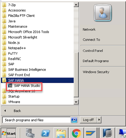
- You have installed SAP HANA Studio on your PC.
Before you start:
- After installing the SDI Agent or SAP HANA Data Provisioning agent you will need to perform the initial configuration.
- To do so, open the administration tool.
- Click on “Connect to HANA” and specify the required details (hostname, port, user and password). Optionally the connection can be established using SSL.
- After confirming, make sure that the “Status” is “Connected”.

- Now you will be able to deploy and register the required adapters. In our example we will use the “ExcelAdapter”. Make sure that this adapter is deployed and registered to SAP HANA.

- In the menu, choose Configure and select the option Preferences to adjust the settings. For example, under Adapters and then ExcelAdapter you can set an access token to protect the access.
- By default, all the file adapters use the agent installation folder to read files. In our example the agent is installed on a Windows server and the path for the excel adapter is “C:\usr\sap\dataprovagent\excel”.
- In our example, the main folder contains multiple subfolders and the Excel file we will use as a source is stored in one of these subfolders.
- A copy of the source file we will be using for this example is published in this link. You can use the file to reproduce this example in your own system.
Steps:
Step1: Remote source and virtual table creation
- First, you will need to note down the name of the staging tables of the migration project and specific migration objects you want to migrate.
- You can find the names of the staging tables for your migration project on the Migration Object Details screen → Staging Tables. The table names are showed in the column called “Staging Table”.
- For detailed information, see: https://help.sap.com/viewer/81152a97f8394fb6bffd19a5632be2e3/latest/en-US/a9dceda5804042b0a49ea9f61c...
- For this exercise, you will need to note down some table names because we will need this information later when creating the data flow object.

- Note down the table names for:
- General Data
- BP Roles.

- Open your SAP HANA studio and select the Administration Console.
- Connect to the SAP HANA database you want to use for staging tables.
- Now you will create the remote source connected to the agent already installed. To do this, expand the folder “Provisioning”.
- Right-click on the “Remote Sources” folder and select “New Remote Source…”.

- Provide a name for the remote source.
- Select the adapter name “ExcelAdapter”.
- Specify the name of the subfolder that the agent will check.
- Provide the additional parameters depending on the file. For example, in our case the property “First Row as Header” is “true” and for “Start Row of Data” is also set to 2.
- Specify the user token value if you have previously configured this in the provisioning agent.
- Fill all the mandatory remaining fields with dummy values (for example “test”).
- Note: SharePoint Credentials are not relevant in this case but, the interface makes them mandatory.
- Choose on the top right corner to save and activate the object.

- Now in the column on the left expand the folder “Remote Sources” and you will find the remote source you have just created.
- If you now expand the connection, you will see the list of Excel files available in the folder you configured. In our example we have 2 files.

- If you select the corresponding xlsx file (loaded previously in the source folder) you will see all sheets available in the form of different tables.

- In our example, the Excel file contains just one sheet and for this reason you can see only 1 table inside.
- If you right-click on one of the tables and choose “Add as Virtual Table” it will add this as a virtual table in your own schema and then you will be able to access the data.

- Make sure that the schema selected is the correct one.
- Define a name for the table or leave the proposal.
- Choose “Create” to start the table creation.

- Once the table has been created, you can now check the content.
- Go to the folder “Catalog” and expand the user/schema you previously selected.
- Right-click on folder “Tables” and choose “Refresh”. Now you should see the virtual table you just created.
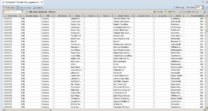
- Right-click the table and choose “Open Data Preview” to check the content. You will see that there are different column corresponding to the different column on the file Excel.

- Browse the content to check the available data.
- NOTE: Before we can proceed with the steps you will need to assign special authorisations for your schema to the technical user “_SYS_REPO”, since this user will be responsible for technically executing the data replication and therefore needs to be able to read from the virtual table you just created in your schema.
- To do this, navigate to Security > Users and double-click the _SYS_REPO user.

- In the user, open the tab “Object Privileges” and hit the button “+” to add a privilege.
- In the pop-up search for your user ID (for example TRAININGA01) and select the schema you want.
- Choose “OK” to confirm the selection.

- Navigate back to the object privileges tab and select the privilege “SELECT” from the list on the right and choose the option “Yes” on the right to make the privilege grantable to others.
- Save by choosing the button in the top right corner.

Now that the data from the source file is available as a virtual table in SAP HANA and the authorisations are correctly set, you can create a Flow Graph object to transfer this data from the virtual table into the staging tables created previously by the Migration Cockpit.
Step2: Flow Graph creation and mapping
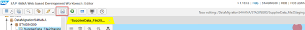
- From the browser access to the SAP HANA Web-based Development Workbench Editor. The url has the following schema:
- http://<full hostname>:80<XX>/sap/hana/ide/editor/ (where <XX> is the system number)
- Login with your SAP HANA user and password.
- Create a new package to store the new objects or reuse an existing one.
- Right-click the package you would like to use and select “New” >> “Flow Graph”.

- Specify a name for the new flow graph. For example: “SupplierData_File2Staging”. Choose “Create” to confirm.
- First drag and drop the function “Data Source” under “General” from the left panel into the content area in the middle.
- At this point the system displays a pop-up requesting for the source table.
- Select the virtual table you previously created from your user schema (in our example STUDENTA01 >> Tables >> STUDENTA01_SupplierData). Choose “OK” to confirm.

- Now you will include the 2 target tables you previously noted down from Migration Cockpit to the content area.
- To do this, select the function Data Sink from the left column.
- When you drop this into the content you will see a pop-up asking for the table name. Select the table corresponding to General Data (as previously noted down) from schema “STAGING_MASTER”.
- NOTE:If you don’t know the table name you can check the Migration Cockpit in the object Supplier where you will find a table name for every structure in the object.

- NOTE:If you don’t know the table name you can check the Migration Cockpit in the object Supplier where you will find a table name for every structure in the object.
- Add another “Data Sink” function and select the table corresponding to structure “BP Roles” (as previously noted down) from the related schema (in our example “STAGING_MASTER”).
- Now you can add an intermediate node that you will use to filter and transform the source data.
- Select the node “Filter” from the left panel and add this to the content area between the source and the target tables.

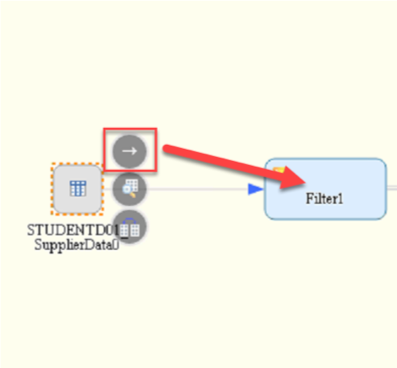
- Now you will create the connections between the block to generate the data flow.
- Select the source table and then the icon with the arrow. Drag the arrow to the filter block to create a connection.
- Double-click the block Filter1 you just added.
- Now you should see the options and configurations for the filter.
- By default, the node is configured to transfer all the source columns to the target. You will need to change this configuration.
- In the right column called “Output”, there are two icons on each row. One icon to change and another to delete the row.

- Select the “Vendor Key” in the right column (Output) and choose the pencil icon. Select the data type as “NVARCHAR”. Set the length as 80. Choose OK to confirm.

- Make sure that “Vendor Key” is still selected in the right column (Output).
- In the lower part of the screen, there is a box called “Node Details”. In the mapping tab choose the button “Expression Editor”.
- Use the function TO_NVARCHAR to convert the number to a string. You can select the function from the Functions column in the category “Conversion Functions”. Choose “OK” to confirm.
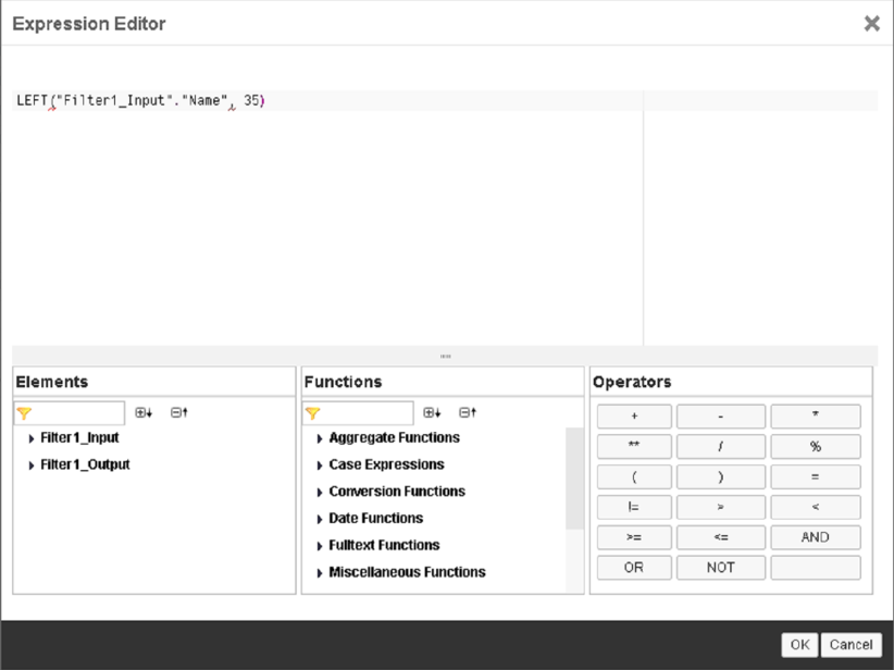
- Select the “Name” in the right column (Output) and choose the pencil icon. Select the Data Type as “NVARCHAR”. Set the length as 35. Choose OK to confirm.

- Make sure that “Name” is still selected in the right column (Output).
- In the lower part of the screen, there is a box called “Node Details”. In the mapping tab choose the button “Expression Editor”.
- Set the expression: LEFT (“Filter1_Input”.”Name”, 35)
- NOTE: This takes only the first 35 characters of the string.
- NOTE: This takes only the first 35 characters of the string.
- You can select the function from the “Functions” column in the category “String Functions”. Choose “OK” to confirm.
- Select the “Search Term 1” in the right column (Output) and choose the pencil icon. Set the length as 20. Choose OK to confirm.
- Make sure that “Search Term 1” is still selected in the right column (Output).
- In the lower part of the screen there is a box called “Node Details”. In the mapping tab choose the button “Expression Editor”.
- Set the expression: LEFT(“Filter1_Input”.”Search Term 1”,20)
- NOTE: Use of function LEFT gets only the first 20 characters of this column. You can select the function from the Functions column in the category “String Functions”.
- Choose “OK” to confirm.
- Select the “House Number” in the right column (Output) and choose the pencil icon. Select the Data Type as NVARCHAR. Set the length as 10. Choose OK to confirm.
- Make sure that “House Number” is still selected in the right column (Output). In the lower part of the screen there is a box called “Node Details”. In the mapping tab, choose the button “Expression Editor”.
- NOTE: Use of function TO_NVARCHAR converts the number to a string. You can select the function from the Functions column in the category “Conversion Functions”. Choose “OK” to confirm.
- Select the “Building” in the right column (Output).
- In the lower part of the screen, there is a box called “Node Details”. In the mapping tab choose the button “Expression Editor”.
- Set the expression: CASE WHEN “Filter1_Input”,”Building” IS NULL THEN ‘ ‘ ELSE “Filter1_Input”.”Building” END
- NOTE: With the function CASE you avoid transferring null values to the target and then function TO_NVARCHAR to convert the number to a string. This expression ensures that null values are transferred to the target field as empty values if the target field does not accept null values. Choose “OK” to confirm.

- NOTE: With the function CASE you avoid transferring null values to the target and then function TO_NVARCHAR to convert the number to a string. This expression ensures that null values are transferred to the target field as empty values if the target field does not accept null values. Choose “OK” to confirm.
- Select the “Floor” in the right column (Output) and choose the pencil icon. Select the data type as NVARCHAR. Set the length as 10. Choose OK to confirm.
- Make sure that “Floor” is still selected in the right column (Output). In the lower part of the screen, there is a box called “Node Details”. In the mapping tab choose the button “Expression Editor”.
- Set the expression: CASE WHEN “Filter1_Input”.”Floor” IS NULL Then ‘ ‘ ELSE TO_NVARCHAR(“Filter1_Input”.”Floor”), END
- NOTE: With the function CASE to avoid that mull values will be transferred to the target and then function TO_NVARCHAR to convert the number in a string. This expression makes sure that in case of null an empty value is transferred to the target field that is not nullable and would not accept null as value. Choose “OK” to confirm.

- NOTE: With the function CASE to avoid that mull values will be transferred to the target and then function TO_NVARCHAR to convert the number in a string. This expression makes sure that in case of null an empty value is transferred to the target field that is not nullable and would not accept null as value. Choose “OK” to confirm.
- Now you will delete the columns that are not required since they are empty in the source structure.
- To do this, you will need to select the corresponding “Field Name” in the right column (Output) and choose the icon representing a bin to delete the row and then choose “OK” to confirm the column deletion. Execute this procedure for the following output fields: First Name, Name 3, Name 4, Search Term 2, Group Key, Different City, State, Transportation Zone, Room, C/O Name, Street 2, Street 3, Supplement, Street 4, Street 5, Tax Jurisdiction Code, PO Box, Postal Code 2, Company Postal Code, URI Type, URI, Central posting block, Purchasing block.
- Choose the button “Back” to return in the main flow graph.
- Now you will connect the filter to the target table.
- Select the filter block and after click and hold on the icon with the arrow to create the connection to the first table you imported corresponding to “General Data”.

- In the content area double-click on the first target table corresponding to “General Data”.
- NOTE: The table name and number will be different than the one in the screenshot.

- NOTE: The table name and number will be different than the one in the screenshot.
- Now you will define the mappings. To do this, drag and drop the columns from the left to the right list.
- In the following pictures you can see the different mappings. When completed a section you will need to scroll down on the source and target to continue with the mapping.
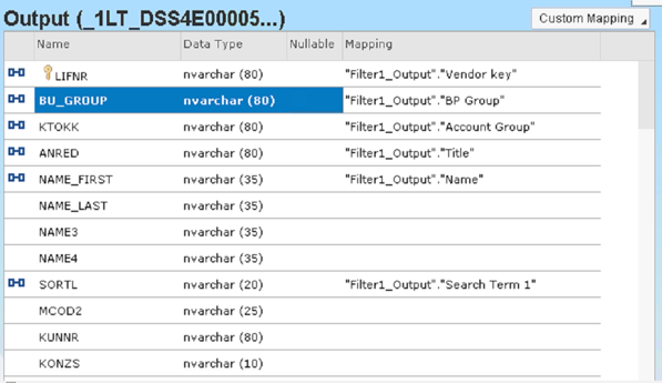


- Make sure to include the following mappings:
- Vendor Key >> LIFNR
- BP Group >> BU_GROUP
- Account Group >> KTOKK
- Title >> ANRED
- Name >> NAME_FIRST
- Search Term 1 >> SORTL
- Street >> STREET
- House Number >> HOUSE_NUM1
- District >> CITY2
- Postal Code >> POST_CODE1
- City >> CITY1
- Country >> COUNTRY
- Time Zone >> TIMEZONE
- Building >> BUILDING
- Floor >> FLOOR
- Language >> LANGU_CORR
- Telephone >> TELNR_LONG
- Mobile >> MOBILE_LONG
- Fax >> FAXNR_LONG
- Email >> SMTP_ADDR
- Click now the button “Back” to return in the main flow graph.
- Now you will work on the mapping of the „BP Roles“ part. To do this you need to load all the supplier numbers together with the 2 corresponding roles.
- Let’s start with the first one: drag and drop a new “Filter” operation in the canvas.
- Connect the source table to the filter directly and double click on the filter to open it and change the content.
- Rename the node as “BP_Roles_1”.

- Delete all the target values on the right except for Vendor Key and BP Group.
- NOTE: If you are wondering if the is a quicker way to delete them not one by one unfortunately there is not. So you will need to select every field and click the deletion icon confirming the pop-up with yes.
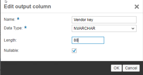
- The result you should have is the one showed in the picture. Now click on the change icon corresponding to the field Vendor Key.

- Set Data Type to NVARCHAR. Specify Length as 80. Click OK.
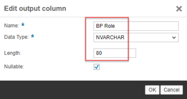
- Now click on the change icon corresponding to the field BP Group.
- Change the Name to BP Role. Verify Data Type is NVARCHAR. Change Length to 80. Click OK to Save.
- Now select the target field Vendor Key in the right column and in the Mapping specify the following: TO_NVARCHAR("BP_Roles_1_Input"."Vendor key")
- NOTE: This will convert the integer in input a an NVARCHAR.
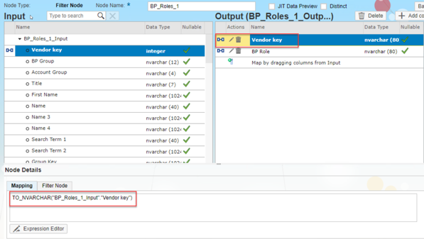
- NOTE: This will convert the integer in input a an NVARCHAR.
- Now select the field BP Role in the right column and replace the mapping with the following constant: 'FLVN00'. NOTE: This is the first role we want to assign.

- Come back to the main canvas by hitting button “Back”.
- Now you will manage the second role. Add a new filter node in the canvas and connect the source table to it.
- Double click on the new node. Rename the node as “BP_Roles_2”.

- Delete all the target values on the right except for Vendor Key and BP Group as you did for the previous filter node.
- The result you should have is the one showed in the picture. Now click on the change icon corresponding to the field Vendor Key

- Set Data Type to NVARCHAR. Specify Length as 80. Click OK.
- Now click on the change icon corresponding to the field BP Group. Change the Name to BP Role. Verify Data Type is NVARCHAR. Change Length to 80. Click OK to save.
- Select the target field Vendor Key in the right column and in the Mappping specify the following: TO_NVARCHAR("BP_Roles_2_Input"."Vendor key")
- NOTE: This will convert the integer in input a an NVARCHAR.
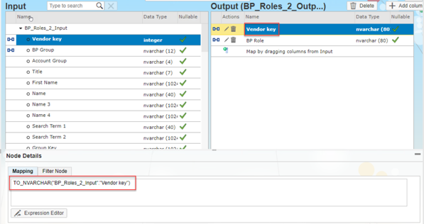
- Select the field BP Role in the right column and replace the mapping with the following constant: 'FLVN01'
- NOTE: This is the first role we want to assign.

- Now you can come back to the previous screen by hitting button “Back”.
- You will need now to put together the 2 outputs in the same result (with 2 columns) using a union.Add a new node Union in the canvas and connect the 2 filters you just created (BP_Roles_1 and BP_Roles_2) to it.

- Double-click on the new Union node and change the Node Name to BP_Roles_All.
- The fields are already automatically mapped because you used the same field names in both the filter outputs.
- Come back to the previous screen by hitting button “Back”.
- Connect the node BP_Roles_All to the second target table that is not yet connected (corresponds to the BP Roles).

- Double click on the table name that you just connected. Here drag and drop the fields from left to right in the following way:
- Vendor Key to LIFNR
- BP Role to BP_ROLE

- The result you should have in the canvas is the same showed in this picture.

- Choose the button to save the object. This will also automatically activate the object and generate the runtime. If the button is grey right click on the object from the left column and select “Activate”.
- Check in the terminal window in the bottom (black background) that the activation happens successfully.

Step 3: Load the data to the staging tables
- Now that the object is active you can execute the data transfer.
- To do this, choose the Execute button.

- Check that the execution is completed successfully in the terminal window on the bottom of the screen.
In case of errors follow the next steps.
HINT. If you get an error during the execution, first check and solve the issue. After this you need to empty the staging tables before re-executing the data flow.
Why? You do that because a partial execution of the flow can have already filled some tables but not all and if you re-execute immediately it will result in an inconsistency generating a duplicate key error.
- In order to check and solve the issues (in case of any) go to the Migration Cockpit and open your migration object and check the 2 tables you used in the mapping by looking at the last column “Number of Records”. Select the tables with existing records and choose Open.
- In the next screen using the processing status you can check the content (select Unprocessed to see the data).
- You now need to choose the button “Delete All Records” to empty the table.

- Now you can execute again the flow.
You can now check the content of your table directly from the object.
- In the content area, select the first target table and you will see a lens icon. Click on this icon to see the content of the table.

- Do the same on the other tables to verify the result.
Step 4: Import the data in SAP S/4HANA using Migration Cockpit
After finishing all these steps, you will have successfully loaded the data from the virtual table (connected to the excel file) into the staging tables.
The next step is now to import the data in SAP S/4HANA using Migration Cockpit and starting the data transfer.
The forth and final blog post of this blog series will focus on SAP HANA Studio – Data from File option.
See an overview of the complete blog series:
Part 1: Migrating data using staging tables and methods for populating the staging tables
Part 2: Using SAP Data Services to load data to the staging tables
Part 3: Using SAP HANA Smart Data Integration (SDI) to load data to the staging tables (this post)
Part 4: SAP HANA Studio – Data from File option
- SAP Managed Tags:
- SAP S/4HANA,
- SAP S/4HANA migration cockpit,
- SAP S/4HANA Cloud Public Edition
Labels:
4 Comments
You must be a registered user to add a comment. If you've already registered, sign in. Otherwise, register and sign in.
Labels in this area
-
Artificial Intelligence (AI)
1 -
Business Trends
363 -
Business Trends
29 -
Customer COE Basics and Fundamentals
1 -
Digital Transformation with Cloud ERP (DT)
1 -
Event Information
461 -
Event Information
28 -
Expert Insights
114 -
Expert Insights
189 -
General
1 -
Governance and Organization
1 -
Introduction
1 -
Life at SAP
414 -
Life at SAP
2 -
Product Updates
4,679 -
Product Updates
275 -
Roadmap and Strategy
1 -
Technology Updates
1,499 -
Technology Updates
100
Related Content
- EXTRACTING DATA FROM SAP S/4HANA CLOUD USING THE CUSTOMER DATA RETURN APP AND TRANSFERRING IT in Enterprise Resource Planning Blogs by SAP
- EHS Data Migration for SAP S/4hana on-premise in Enterprise Resource Planning Q&A
- SAP Activate Realize and Deploy phase activities in the context of Scaled Agile Framework in Enterprise Resource Planning Blogs by SAP
- Preferred Success Round Table Discussion with SAP Customers on 29th April @ SAP NOW India. in Enterprise Resource Planning Blogs by SAP
- Adding Custom Fields to Migration Objects in SAP S/4HANA Cloud Public Edition in Enterprise Resource Planning Blogs by SAP
Top kudoed authors
| User | Count |
|---|---|
| 7 | |
| 6 | |
| 4 | |
| 4 | |
| 4 | |
| 4 | |
| 3 | |
| 3 | |
| 3 | |
| 3 |