
- SAP Community
- Products and Technology
- Technology
- Technology Blogs by SAP
- SAP BTP Data & Analytics Showcase - Data Preparati...
Technology Blogs by SAP
Learn how to extend and personalize SAP applications. Follow the SAP technology blog for insights into SAP BTP, ABAP, SAP Analytics Cloud, SAP HANA, and more.
Turn on suggestions
Auto-suggest helps you quickly narrow down your search results by suggesting possible matches as you type.
Showing results for
Employee
Options
- Subscribe to RSS Feed
- Mark as New
- Mark as Read
- Bookmark
- Subscribe
- Printer Friendly Page
- Report Inappropriate Content
12-06-2021
8:37 AM
Introduction
This is the first part of the blog series "SAP BTP Data & Analytics Showcase - Empower Data Scientist with Flexibility in an End-to-End Way". In this blog post, we'd like to demonstrate how to prepare data in a typical data science scenario, taking advantages of different capabilities in SAP Data Warehouse Cloud, e.g., federation & replication, self-service modelling and seamless integration with SAP Analytics Cloud.
The overall implementation steps are demonstrated as follows:
- Connect and collect necessary data from different sources into SAP Data Warehouse Cloud
- Prepare training data set using self-service modelling capabilities, e.g., graphical view or SQL view builder - (consumed later in Jupyter Notebook)
- Create analytical data set to show historical price changes from 2017 to 2021 - (visualised later in SAP Analytics Cloud)

Fig.1: High-level Solution Overview in SAP Data Warehouse Cloud
Part 1: Collect and connect data from different sources
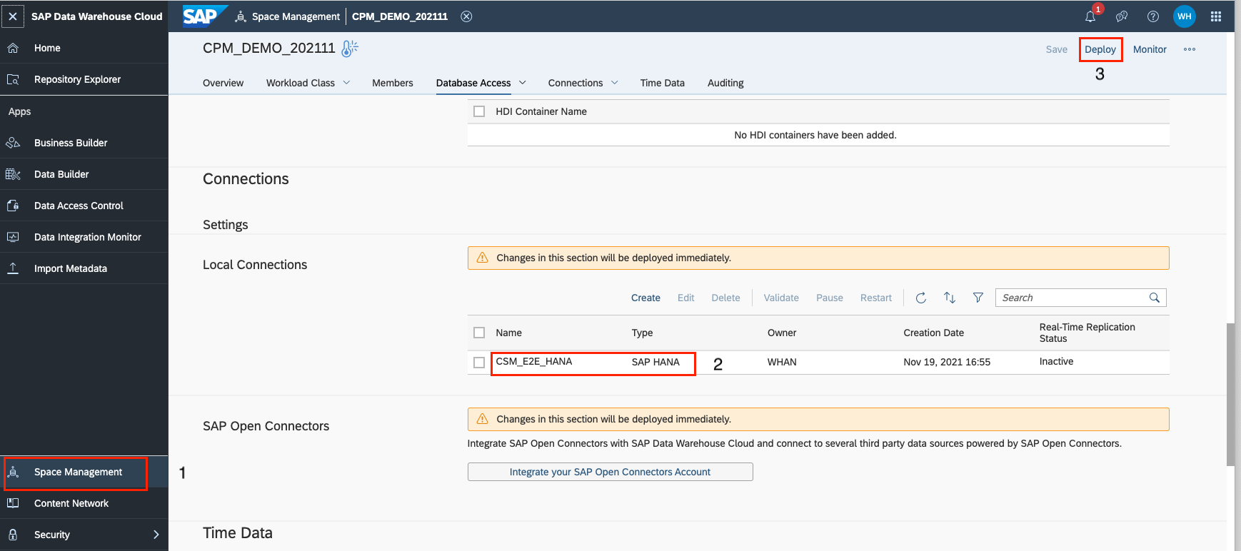
Step 1: Create a connection
First of all, we created a space under SAP Data Warehouse Cloud and a local connection called "CSM_E2E_HANA" to access a SAP HANA Cloud tenant. After saving the configuration, you need to click on the "Deploy" button to make the changes effective. You can go to this document for more details.
Step 2: Import tables from SAP HANA Cloud
To enable Federation Query to tables (e.g., historical prices) located in SAP HANA Cloud, we navigate to "New Graphical View" under Data Builder and import remote tables in the repository of SAP Data Warehouse Cloud. You can achieve it easily by drag and drop tables into the canvas of graphical view builder. The same steps can be taken for other three tables from SAP HANA Cloud.

Step 3: Import CSV files
By pressing the "import" button, you're able to choose the "Import CSV File" option and load COVID-19 data of Baden-Württemberg into SAP Data Warehouse Cloud.

Afterwards, you have the possibility to modify the imported CSV data, e.g., rename columns or convert data types, as it is deployed as "local table" in SAP Data Warehouse Cloud.

As of now, you have integrated all the necessary data into one central place. The following tables shall be displayed in your Data Warehouse Cloud tenant:

Part 2: Prepare training dataset using self-service modelling
As a next step, we'll utilise self-service modelling features in SAP Data Warehouse Cloud to build a harmonised view (relational dataset), which works as training data and can be accessed via Jupyter Notebook later.
Step 1: Create a basic view combining necessary data
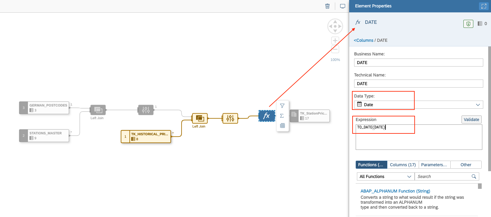
First of all, a view called "TK_StationPrices_Historical" was established (see Figure 1), which combines station master, historical prices and federal states data.

What we love like to highlight here: It is quite convenience to create calculated columns in SAP Data Warehouse Cloud, with help of simplified user interfaces. For instance, the column "DATE" was converted as a calculated column in my case, which calculates the DataTime type (2017-02-28 07:45:31.000000000) to Date type (2017-02-28), as we are interested in the daily-based prices, not hourly.
You can follow the implementation steps in the below video and build your own data model in 5 minutes.
Step 2: Create training data set for forecasting multiple time-series
In this part, we would like to demonstrate how to prepare training data set for ML part. Our objective is to predict the next 7 days gasoline prices, taking the factor of COVID-19 situation into account.
To achieve this goal, Forecasting Multiple Time-Series is applied in this use case. On one hand, we have the historical gasoline prices from different federal states (e.g., Baden-Württemberg) from the above-created view "TK_StationPrices_Historical". On the other hand, COVID-19 data, e.g., case number, is also available in this website by RKI, which is also organised by federal state in Germany. So, we decided to use these two kind of data as my training data and pursue an individual time-series forecasting based on federal state.
In the end, our target training data set should look like as follows (data in this table is only example, may be not 100% correct): One record for one federal state on one day.

1. Create an aggregated view showing Average Gasoline Prices per Federal State per Day
We got all the historical prices data from stations in Germany, during various time of a specific day from 2017 to 2021. Therefore, it is better to create an aggregated view to represent the gasoline prices (Diesel, Super E5 and Super E10) for each federal state on an individual day. Let's navigate to the SQL View Builder of SAP Data Warehouse Cloud and create a SQL view called "TK_StationPrices_Avg".
You are able to complete this step by parsing the following SQL statement shown below.
SELECT "DATE",

	"STATE",

	AVG("DIESEL") AS "DIESEL",

	AVG("E5") AS "E5",

	AVG("E10") AS "E10",

	AVG("DIESELCHANGE") AS "DIESELCHANGE",

	AVG("E5CHANGE") AS "E5CHANGE",

	AVG("E10CHANGE") AS "E10CHANGE"

FROM "TK_StationPrices_Historical"

GROUP BY "DATE",

	"STATE"
2. Create an aggregated view showing Total Cases, New Cases and Recovered Cases
In this demo, COVID-19 data for federal state "Baden-Württemberg" was downloaded and used as an example. This is one time-series forecasting. The same implementation can be done for other federal states.
Another SQL view was created based on the imported COVID-19 data, which shows us, for instance, total case numbers and total new cases on a specific day inside Baden-Württemberg, from February 2020 till now.
SELECT "Meldedatum",

	"Bundesland",

	SUM("NeuerFall") AS "NewCase",

	SUM("AnzahlFall") AS "TotalCase",

	SUM("AnzahlGenesen") AS "RecoveredCase"

FROM "RKI_COVID19_BW"

GROUP BY "Meldedatum",

	"Bundesland"
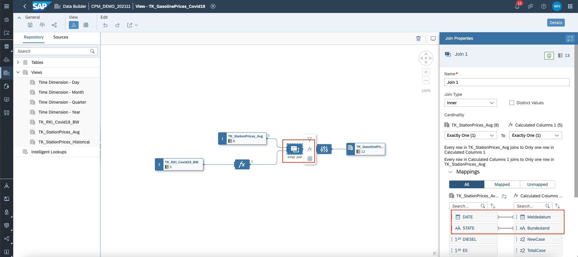
3. Combine Average Gasoline Prices with COVID-19 Cases
As a last step, we'd like to combine the two SQL views into one relational dataset via Graphical View Builder, which represents my target training dataset as well. In addition, we can look at the final training dataset using Data Preview together.

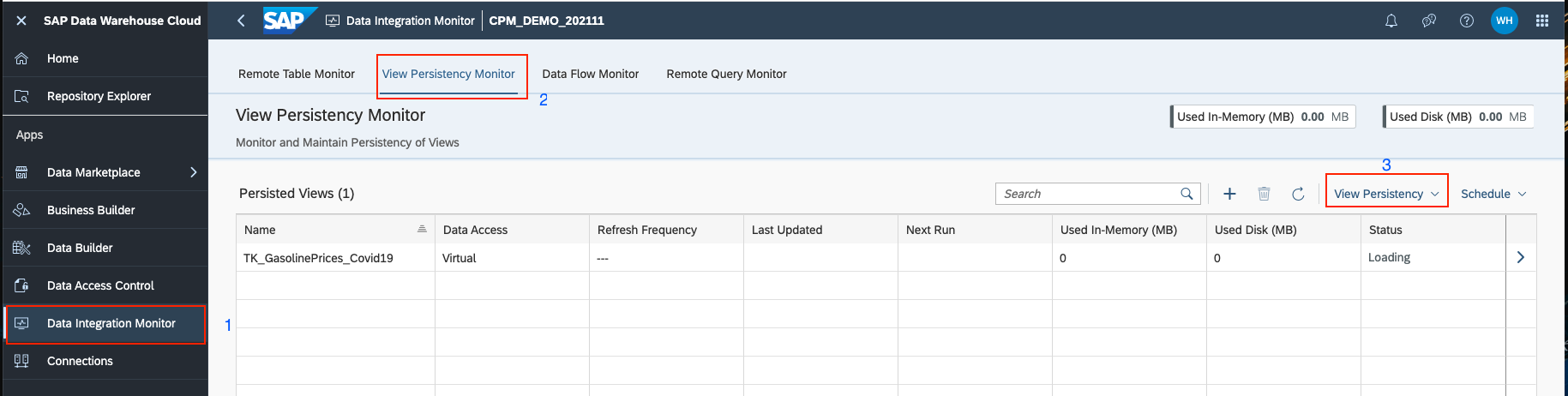
Step 3: (Optional) Persist a view using Data Integration Monitor
To improve performance to access data from different sources, you have the opportunity to persist your views through Data Integration Monitor in SAP Data Warehouse Cloud. This is an optional step.

Part 3: Create analytical data set to show historical price changes from 2017 to 2021
To help data scientists better understand the historical price changes and visualise their findings in the end, a dashboard was created in SAP Analytics Cloud. In this dashboard, a story was established to illustrate:
- Historical Prices Trend Change from 2017 to 2021
- Comparison of Gasoline Prices during Holidays in Germany (2020 vs 2021).
For this purpose, an analytical dataset was created in SAP Data Warehouse Cloud, which was used as a data source for story in SAP Analytics Cloud.
Step 1: Create time dimension under Space
To illustrate the historical prices flexibly, let's leverage the "Time Dimension" capability in SAP Data Warehouse Cloud. This means, time-related views, e.g., calendar month and calendar year, are created automatically for a defined period and used later in your data models. You're able pursue this step under your Space and find related views in your Data Builder.


Step 2: Build analytical data set via Graphical View Builder
To visualise the time-related information in my story, e.g., gasoline prices per calendar month, we joined the view "TK_StationPrices_Historical" with the view "Time Dimension - Day". To compare the gasoline prices (2020 vs 2021) during various holidays in Germany, the table "German_Holidays" was added to the canvas too. Finally, I selected the gasoline prices as measures and configured them. Here, we chose the maximal prices.
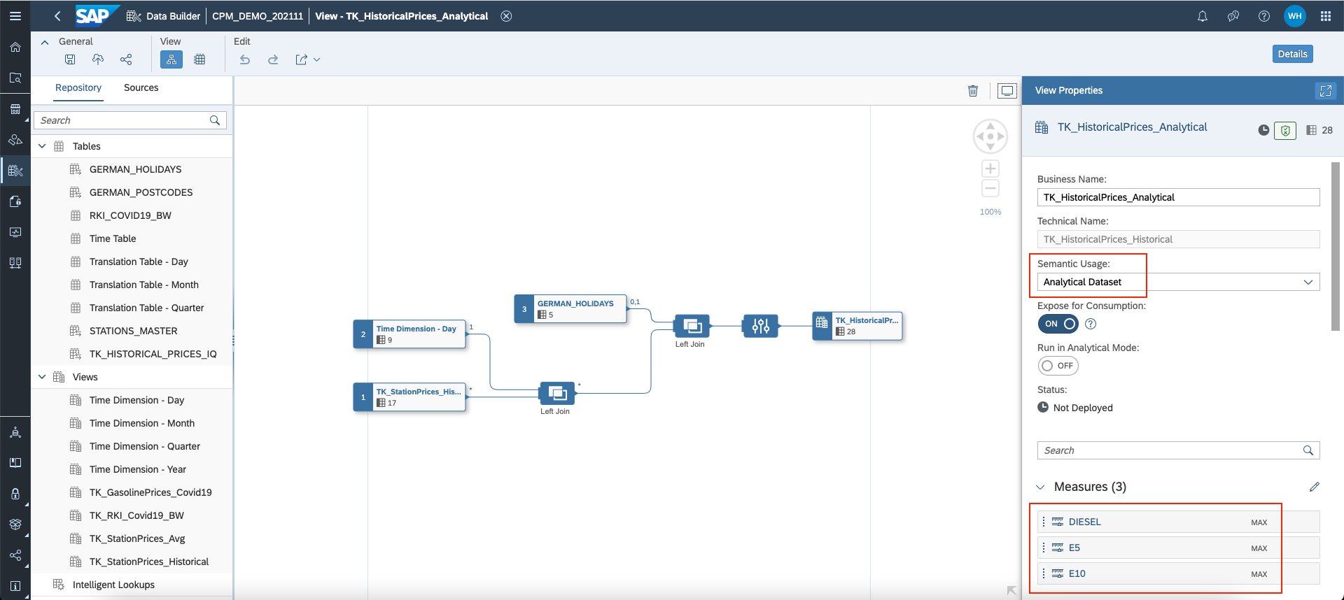
Now, let's have a look together how the analytical data set looks in the Data Preview. It combines the necessary information we need - gasoline prices, German holidays and time dimensions.

Step 3: Visualise results
In SAP Analytics Cloud, we can choose this analytical data set as data source and start to build our report. In this blog post, I'll not demonstrate the implementation in SAP Analytics Cloud. Instead, we'd like to share these two charts, which help data scientists visualise their findings in a way that business users or other audience can easily understand.

Trend Chart: Gasoline Price Changes in Germany based on Calendar Month during 2017 and 2021

Comparison Chart: Gasoline Price Comparison during Holiday in Germany (2020 vs 2021)
Conclusion
We understand data preparation is quite an essential part for any data science project. We hope this blog can give a comprehensive insights about how capabilities of SAP Data Warehouse Cloud can help data scientist experts prepare data in a self-service, simplified and flexible way. Additionally, we take your pain point about visualisation of your findings in an understandable way into consideration. We demonstrate how the seamless integration between SAP Data Warehouse Cloud and SAP Analytics Cloud can help data scientists show results to business users or other audience more easily.
Hope you enjoyed this blog post! If you are curious about how to access the training data in Jupyter Notebook and create ML models, please move to the 2nd blog post of this blog series.
- SAP Managed Tags:
- SAP Analytics Cloud,
- SAP Datasphere,
- SAP HANA Cloud,
- SAP Business Technology Platform
Labels:
3 Comments
You must be a registered user to add a comment. If you've already registered, sign in. Otherwise, register and sign in.
Labels in this area
-
ABAP CDS Views - CDC (Change Data Capture)
2 -
AI
1 -
Analyze Workload Data
1 -
BTP
1 -
Business and IT Integration
2 -
Business application stu
1 -
Business Technology Platform
1 -
Business Trends
1,658 -
Business Trends
112 -
CAP
1 -
cf
1 -
Cloud Foundry
1 -
Confluent
1 -
Customer COE Basics and Fundamentals
1 -
Customer COE Latest and Greatest
3 -
Customer Data Browser app
1 -
Data Analysis Tool
1 -
data migration
1 -
data transfer
1 -
Datasphere
2 -
Event Information
1,400 -
Event Information
74 -
Expert
1 -
Expert Insights
177 -
Expert Insights
348 -
General
1 -
Google cloud
1 -
Google Next'24
1 -
GraphQL
1 -
Kafka
1 -
Life at SAP
780 -
Life at SAP
14 -
Migrate your Data App
1 -
MTA
1 -
Network Performance Analysis
1 -
NodeJS
1 -
PDF
1 -
POC
1 -
Product Updates
4,575 -
Product Updates
391 -
Replication Flow
1 -
REST API
1 -
RisewithSAP
1 -
SAP BTP
1 -
SAP BTP Cloud Foundry
1 -
SAP Cloud ALM
1 -
SAP Cloud Application Programming Model
1 -
SAP Datasphere
2 -
SAP S4HANA Cloud
1 -
SAP S4HANA Migration Cockpit
1 -
Technology Updates
6,871 -
Technology Updates
483 -
Workload Fluctuations
1
Related Content
- Watch the SAP BW Modernization Webinar Series in Technology Blogs by SAP
- First steps to work with SAP Cloud ALM Deployment scenario for SAP ABAP systems (7.40 or higher) in Technology Blogs by SAP
- What’s New in SAP Datasphere Version 2024.10 — May 7, 2024 in Technology Blogs by Members
- Unveiling SAP Analytics Cloud Performance Analysis Insights for Optimal Performance in Technology Blogs by Members
- "Replace Model" Feature in SAP Analytics Cloud with SAP BW Live Model in Technology Blogs by Members
Top kudoed authors
| User | Count |
|---|---|
| 14 | |
| 11 | |
| 10 | |
| 10 | |
| 9 | |
| 8 | |
| 7 | |
| 7 | |
| 7 | |
| 7 |