
- SAP Community
- Products and Technology
- Technology
- Technology Blogs by SAP
- Connecting to SAP HANA Service from Anywhere
Technology Blogs by SAP
Learn how to extend and personalize SAP applications. Follow the SAP technology blog for insights into SAP BTP, ABAP, SAP Analytics Cloud, SAP HANA, and more.
Turn on suggestions
Auto-suggest helps you quickly narrow down your search results by suggesting possible matches as you type.
Showing results for
Former Member
Options
- Subscribe to RSS Feed
- Mark as New
- Mark as Read
- Bookmark
- Subscribe
- Printer Friendly Page
- Report Inappropriate Content
11-06-2018
4:41 AM

SAP HANA as a Service is a fully managed service, available in the SAP Cloud Platform. While it is fairly obvious that you can use SAP HANA as a Service with all the other SAP Cloud Platform Services to develop data driven applications, I will use this post to talk about how you could use the SAP HANA service instance with any other development environment.
For SAP TechEd 2018, I was asked to construct a way to showcase this. Before we begin, here is a high-level overview of the essential technologies and tools that will be used in this demo:
- SAP HANA as a Service instance – SAP HANA as a managed cloud service
- Windows running on an AWS EC2 instance – Amazon’s virtual machine where users can run their own applications
- SAP Python driver (hdbcli) – Python driver that allows a connection to SAP HANA from a Python application
Here are the following technologies and tools that are specific to this Python application:
- Kaggle – a data science community with freely accessible data sets
- Why: Kaggle has free and publicly available data sets, which we could import into the SAP HANA Service instance
- Anaconda – a Python data science platform that packages the newest Python edition and Jupyter notebook
- Why: allows us to install all the necessary Python tools in one place
- Jupyter Notebook – Python environment used for data analysis and data science
- Why: allows us to document and code in the same environment
- Pandas – Python mathematical data analysis library
- Why: allows us to take datasets and put them into frames to aggregate, chart, and map out data
- Matplotlib – Python 2D plotting library
- Why: allows us to generate simple charts from a dataset from with a few lines of code
There are a few prerequisites for this demo I’ll briefly go over now. The first prerequisite is a running AWS EC2 instance with a Windows OS. This instance that I used is a t2.micro instance which can be changed depending on your needs. The second prerequisite is a SAP HANA Service instance provisioned through the SAP Cloud Platform with imported data. When setting up the SAP HANA Service instance, it’s recommended that you pre-authorize IP addresses that can establish connections.
NOTE: Kaggle is a great (and free) place to get datasets that can be easily imported into SAP HANA.
The following requirements are application specific. For the purposes of this demo application, we will be working in a Python environment on our AWS EC2 instance. First connect to your AWS EC2 instance and install Python and Jupyter notebook through the Anaconda installation. Create an application folder under documents. Then open the command prompt, navigate to your application folder, and install Pandas and Matplotlib with pip.
pip install pandaspip install matplotlibTo connect to the HANA Service instance through a Python application on AWS EC2, we will need the SAP Python driver. To get the up-to-date version, install the Python driver through the SAP HANA Client installation. If you installed the SAP HANA Client locally, move the SAP HANA Client install package onto your AWS EC2 instance (I used WinSCP). In your application folder in the AWS EC2 instance, install the hdbcli-2.3.119.zip file with pip.
pip install hdbcli-2.3.119.zipNOTE: Here is more information on how to install the Python driver
Launch Jupyter Notebook from the command line.
jupyter notebookOnce Jupyter Notebook starts, navigate to your application folder. Create a new Python 3 notebook by clicking the “New” drop down at the top of the right side of the web page. We need to import the Python driver and the other Python packages/modules into our application. We can do this with the following lines, where the first line is the Python driver import.
from hdbcli import dbapi

import pandas as pd

import matplotlib.pyplot as plt
Note: Run the code with the “Run” button in the tool bar to ensure that the packages were successfully imported. You can do this for each stage in the application.
From there, we need the connection information. Here are the connection details for the Python application.
connection = dbapi.connect(

      address="zeus.hana.prod.us-east-2.whitney.dbaas.ondemand.com",

      port=00001,

      encrypt="true",

      user="EXAMPLE_USER",

      password="EXAMPLE_PASSWORD"

)
The information needed to create a connection can be found on the SAP HANA Service Dashboard. We will need the endpoint connectivity information. See below for where the endpoint connection information can be found.

Within the endpoint there will be an address followed by the port number. For direct SQL connections, the address starts with zeus.hana and the rest of the address differs based on where your instance was launched. The number after the address and colon is the port number which differs per instance. Other information that you will need is a user and its password that can connect to the SAP HANA Service instance. For more connection options check out Tom Slee’s blog post.
NOTE: SAP HANA Service requires an encrypted connection which is why encrypt=”true” is required. Additional fields will be required if the host operating system is not Windows since Windows performs the certificate handling on our behalf.
Once the connection has been made, we can use Pandas to read a SQL query and cluster the data into four simple sections. This can be done many ways but for the sake of simplicity, a SQL query was used.
This SQL query takes the NBA player information dataset within our SAP HANA Service instance and sorts them based on their salary groups.
data = pd.read_sql_query('SELECT COUNT("Salary") as "SALARY GROUPS" \
FROM SYSTEM.NBA_SALARY \
WHERE "Salary" > 20000000 \
UNION \
SELECT COUNT("Salary")\
FROM SYSTEM.NBA_SALARY \
WHERE "Salary" BETWEEN 10000000 and 20000000 \
UNION \
SELECT COUNT("Salary")\
FROM SYSTEM.NBA_SALARY \
WHERE "Salary" BETWEEN 1000000 and 10000000 \
UNION \
SELECT COUNT("Salary")\
FROM SYSTEM.NBA_SALARY \
WHERE "Salary"<1000000', connection)
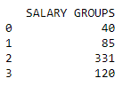
print(data)
This is the result of the SQL query.
From here, labels are created, and a plot is created with Matplotlib using the data gathered.
labels = 'Over 20 million', 'Between 10 and 20 million', 'Between 1 and 10 million', 'Under 1 million'

sizes = data

explode = (0.1,0, 0, 0)

fig1, ax1 = plt.subplots()

ax1.pie(sizes, explode=explode, labels=labels, autopct='%1.1f%%',

        shadow=True, startangle=90)

ax1.axis('equal')

plt.title("NBA Player Salaries in 2017/2018")

plt.show()
This is the plot that was created.

To recap, with minimum software installation and minimum code, we can connect to our SAP HANA Service instance from AWS EC2. The Python environment can be easily changed to a business objects environment, Tableau environment, or any other business intelligence or data science tool.
Here is my Jupyter Notebook as an example.

See below for more resource on this topic.
Rudi Leibbrandt’s live application demo at TechEd Vegas (2018)
Connect to SAP Cloud Platform from Anywhere
More videos on SAP HANA service
SAP HANA Academy – SAP Cloud Platform, SAP HANA Service
GitHub examples
SAPHANAService - GitHub
Kaggle dataset used in the demo
https://www.kaggle.com/koki25ando/salary
- SAP Managed Tags:
- SAP HANA service for SAP BTP
Labels:
3 Comments
You must be a registered user to add a comment. If you've already registered, sign in. Otherwise, register and sign in.
Labels in this area
-
ABAP CDS Views - CDC (Change Data Capture)
2 -
AI
1 -
Analyze Workload Data
1 -
BTP
1 -
Business and IT Integration
2 -
Business application stu
1 -
Business Technology Platform
1 -
Business Trends
1,658 -
Business Trends
103 -
CAP
1 -
cf
1 -
Cloud Foundry
1 -
Confluent
1 -
Customer COE Basics and Fundamentals
1 -
Customer COE Latest and Greatest
3 -
Customer Data Browser app
1 -
Data Analysis Tool
1 -
data migration
1 -
data transfer
1 -
Datasphere
2 -
Event Information
1,400 -
Event Information
69 -
Expert
1 -
Expert Insights
177 -
Expert Insights
326 -
General
1 -
Google cloud
1 -
Google Next'24
1 -
GraphQL
1 -
Kafka
1 -
Life at SAP
780 -
Life at SAP
13 -
Migrate your Data App
1 -
MTA
1 -
Network Performance Analysis
1 -
NodeJS
1 -
PDF
1 -
POC
1 -
Product Updates
4,575 -
Product Updates
374 -
Replication Flow
1 -
REST API
1 -
RisewithSAP
1 -
SAP BTP
1 -
SAP BTP Cloud Foundry
1 -
SAP Cloud ALM
1 -
SAP Cloud Application Programming Model
1 -
SAP Datasphere
2 -
SAP S4HANA Cloud
1 -
SAP S4HANA Migration Cockpit
1 -
Technology Updates
6,872 -
Technology Updates
458 -
Workload Fluctuations
1
Related Content
- Unable to Connect to ABAP Instance from BTP Trial in Technology Q&A
- Authentication of a web service that points to a hana database container in Technology Q&A
- SAP 分析云 2024.09 版功能更新 in Technology Blogs by SAP
- What’s New in SAP Analytics Cloud Q2 2024 in Technology Blogs by SAP
- SAP DS Designer not able to execute a Job in a remote DS Job Server in Technology Q&A
Top kudoed authors
| User | Count |
|---|---|
| 20 | |
| 8 | |
| 8 | |
| 6 | |
| 6 | |
| 6 | |
| 6 | |
| 6 | |
| 5 | |
| 5 |