
- SAP Community
- Products and Technology
- Technology
- Technology Blogs by SAP
- SAP Data Intelligence ABAP Integration with Genera...
Technology Blogs by SAP
Learn how to extend and personalize SAP applications. Follow the SAP technology blog for insights into SAP BTP, ABAP, SAP Analytics Cloud, SAP HANA, and more.
Turn on suggestions
Auto-suggest helps you quickly narrow down your search results by suggesting possible matches as you type.
Showing results for
Product and Topic Expert
Options
- Subscribe to RSS Feed
- Mark as New
- Mark as Read
- Bookmark
- Subscribe
- Printer Friendly Page
- Report Inappropriate Content
02-15-2022
6:02 PM
This is my second part of the blog series about SAP Data Intelligence ABAP integration with generation 2 operators. After going through a lot of theory including prerequisites, concepts etc. for generation 2 ABAP integration in my blog post part 1-Overview and Introduction I will create a real scenario in SAP Data Intelligence using a graph for generation 1 and generation 2 operators in this second blog post. The scenario includes the extraction of data from a custom CDS view located in an SAP S/4HANA 2020 (on-premise) system and loading the data into CSV files in a Google Cloud Storage (GCS) target using initial load and delta load capabilities.
To get started, we first create the required connections that we need for this scenario.
First of all, we need to define the required connections in the Connection Management application pointing to SAP S/4HANA and Google Cloud Storage:
Connection to SAP S/4HANA 2020 using Connection type ABAP and RFC:
Note: In this case the SAP S/4HANA 2020 system has been equipped with all necessary Notes incl. the TCI 3105880.
Connection to Google Cloud Storage (GCS):

CDS view in the source SAP S/4HANA system:
The sample scenario in this blog will use an SAP S/4HANA system (on-premise) and a custom CDS view called “ZCDS_EPM_PO”, which has been created based on the EPM data model that comes with an SAP S/4HANA system. The CDS view is built based on table SEPM_BPA (Business Partners) and has the required Analytics annotations for data extraction + delta extraction as described here: https://help.sap.com/viewer/3a65df0ce7cd40d3a61225b7d3c86703/Cloud/en-US/55b2a17f987744cba62903e97dd...
More information about the EPM data model can be found here: https://help.sap.com/viewer/a602ff71a47c441bb3000504ec938fea/202009.latest/en-US/57e9f59831e94311852...
The design of the graph is quite simple and looks as follows:
Define CDS view extraction
Configure the CDS Reader Operator (here V2 is used) to extract data from CDS view “ZCDS_EPM_PO”.
* This parameter has been introduced recently, and its availability in the operator configuration panel depends on your SAP source system. If your system does not have the latest SAP Notes + TCI Note, this parameter might not be visible for you.
In a second step, a small Python operator is used to extract the CDS view columns out of the header provided in the output message of the CDS Reader operator to generate a CSV stream that contains the CDS view columns in the first row and the actual data body starting in the second line of the CSV data. Therefore, one input port of type message and one output port of type message are used.
There are various ways how to achieve this and you could, for example, pick the following example provided in a blog post by Yuliya Reich: https://blogs.sap.com/2021/02/15/sap-data-intelligence-how-to-get-headers-of-cds-view/. Note that the coding might need to be adjusted depending on your individual use case and the version of SAP S/4HANA you are using.
Code snippet based on Python 3.6:
As a last step the data needs to be loaded to Google Cloud Storage via CSV files. As a necessary prerequisite, the “to File” operator needs to be used as conversion operator to bring the data into the correct format that is required by the Write File operator.
In the Write File Operator configuration panel, we define the following parameters:
In this example file path “/demo/Generation1/ZCDS_EPM_PO/<date>/PO_<time>_<counter>.csv” is using different placeholder functions date, time and counter that will be generated during runtime of a graph whenever a data package is leaving the CDS Reader Operator and will be written into GCS. In this example each incoming data package will be stored and grouped in one folder of the current day, where each file name consists of the prefix “PO_” followed by the time of the data set arrival in the Write file operator and an integer counter that starts with 1 and will be enumerated by +1 for each data set streaming through the graph.
Example: /demo/Generation1/ZCDS_EPM_PO/20220103/PO_071053_1.csv
Please note that when you use the “Create Only” file mode that the placeholders in our example take care of writing all chunks of data into a dedicated file. When you use a plain graph without placeholders and only the first chunk of data will be written to GCS. Technically you can also make use of “Append” file mode, but depending on your scenario an “Append” creating large files might lead to memory problems when large files are created.
There are of course multiple other ways of designing the file name pattern that you can change based on your specific needs. You could for example create your own header information also in python and hand it over to the Write File operator as an input.
As we expect to run the graph 24x7 for initial load and change data capturing we do not add any graph terminator at the end of the graph.
When we now execute the graph, we will see that the following CSV files will be created in Google Cloud Storage as a target using the Metadata Explorer:
Once the initial load is done, there will be one file generated per incoming delta which occurred in the source. This can lead to smaller files being generated in case there is a low number of changes in your source system. Also here you can of course create mechanisms to merge batches into bigger chunks, but in this case, we want to keep it simple.
Now we want to take the same use case we implemented with generation 1 operators to load data from a CDS view to CSV files in Google Cloud Storage and create a graph using the generation 2 operators. The high-level design of the generation 2 graph looks as follows:
1. Define CDS view extraction
In the first part we configure the Read Data from SAP System operator to extract data from CDS view “ZCDS_EPM_PO” using the following configuration parameters:
In our example scenario, we will select the following configurations:
Please note that you should not manually change the displayed value in the Object Name parameter once you selected your data set.
2. Generate binary stream in CSV
Drag and drop the “Table to Binary” operator to the modelling canvas the and connect the output of the Read Data from SAP System operator to the input of the “Table to Binary” operator. The Table to Binary standard operator is required because the Binary Write File operator is requiring a binary input stream. It takes the table-based input from Read Data from SAP System operator and provides different capabilities in which format the data can be further processed, e.g. using CSV, JSON, JSON Lines or Parquet.In our case we select CSV as output format and the following CSV properties:
Note: The “colNames” parameter can be left empty as the column Names will automatically be extracted.
3. Write Partitioned CSV files to Google Cloud Storage
Drag and drop the generation 2 “Binary File Producer” to load the data via CSV files into Google Cloud Storage. Connect the output port “binary” of Table to Binary operator to the input port of the Binary File Producer operator.
In the Binary File Producer operator configuration panel, we define the following parameters:
In this example partitioned files File mode has been selected, which is a necessary prerequisite if we want to use graph resilience feature with snapshots with this operator. As file path parameter I have chosen: “/demo/Generation2/ZCDS_EPM_PO.csv”.
The main difference comparing the Generation 1 graph is that we now have a file mode parameter where we select “partitioned file mode”, which is required for using the snapshot feature. When partitioned file mode is selected, we can currently only define the path up to the partitioned file folder, in this example “ZCDS_EPM_PO.csv”, but not the actual file names of the various part files that are being generated inside our specified folder. The file name pattern is given and by using a generated uuid as well as the batch index that is included in the header information. More information about the handling of files including file name patterns can be checked here: https://help.sap.com/viewer/97fce0b6d93e490fadec7e7021e9016e/Cloud/en-US/64d01ad02e39499594b1eb10397...
There are of course multiple other ways of how you want to store your data in your file storage target system, e.g. using placeholders similar to generation 1 Write File operator in the file path, but in this case we want to keep it simple without using placeholders.
As we expect to run the graph 24x7 for initial load and change data capturing we do not use any graph terminator at the end of the graph.
Spoiler Alert: Usage of last batch and Graph Terminator in initial load mode
Using generation 2 Graphs and Operators there is also an improvement when e.g. using the Initial Load mode in the Read Data from SAP System operator which uses the “isLast” Batch attribute in the header, which is indicating whether the last chunk of data has been loaded from the SAP source system.
In the Graph Terminator operator there is a configuration parameter “On Last Batch”. If we change our graph to perform an “initial Load” in Transfer Mode parameter, add a graph Terminator after the Binary File Producer and set “on Last Batch” to True, the graph will automatically go to completed state when the load is completed:
Furthermore, you could also combine the usage of the Read Data from SAP System operator with structured data operators such as the Data Transform operator, e.g. for performing a projection on the CDS view, which was not possible using the generation 1 operators due to different port types being used by CDS Reader and Data Transform operators:
But now it’s time to execute our graph (using Replication Mode in the Read Data from SAP System operator) .
In the pop-up dialog, you can specify different options:
Note: This parameter specifies whether the automatic restart feature should be used, which is optional. Whenever a graph is failing this feature will take care that the graph is restarted automatically with the maximum number of retries that are specified in “Retry for” within the time interval specified in the “threshold” parameter.
During the start time, you can check the Process Logs tab of your running graph and check out some new metrics that are provided by the generation 2 Read Data from SAP System operator, e.g.

In addition, a new metric for the number of processed records has been introduced for the generation 2 Read Data from SAP System operator:
After the graph status is switching to “running” we can open the Metadata Explorer application to check the files being transferred to Google Cloud Storage.
When we browse inside the directory to the file path we defined “/demo/Generation2/ZCDS_EPM_PO.csv”, we will see that the following directory has been created:
Inside the directory we can now see various part files that were replicated, where each part-file represents one batch of CDS view records. The generated part files follow the naming pattern
“part-<uuid>-<batch_index>.<file_extension>”,
e.g.: part-ffbc63eb-c582-4f90-b3c6-dbeb362e9977-0.csv
We can now also perform a quick data preview for one of the files to check the actual data that has been replicated from SAP S/4HANA to Google Cloud Storage:
Once the initial load is done, there will be one part file generated per incoming delta which occurred in the source. This can lead to smaller files being generated in case there are is a low change rate for the data in the source system. You can of course add mechanisms into your pipeline to merge batches into bigger chunks etc.
With our current configuration of snapshots and auto-restart, the graph will automatically re-start in case of an error and continue the replication using the snapshot information that has been captured at the point of failure.
In case an error happens, you will see in the lower section of the modeler that a new instance of the graph will be started and the failed one will still exist. Both executions are belonging and grouped together under the main graph we started:
Before the error happens, we can see in the Metadata Explorer that up to batch index 5 the CSV files has been generated in Google Cloud Storage:
After the graph successfully restarts, we can see that the replication continues with batch index 6 to continue the replication:
In the overview section of your running or failed graph, you can also check the values you defined upon graph execution as well as the failure count etc.:
Now that’s it. I hope I could give you some useful information about the usage of ABAP integration with SAP Data Intelligence using Generation 2 graphs based on a sample scenario.
Please feel free to add your feedback and question in the comment section of this blog post.
To get started, we first create the required connections that we need for this scenario.
SAP Data Intelligence – Create Connection to SAP S/4 HANA source system & Google Cloud Storage:
First of all, we need to define the required connections in the Connection Management application pointing to SAP S/4HANA and Google Cloud Storage:
Connection to SAP S/4HANA 2020 using Connection type ABAP and RFC:
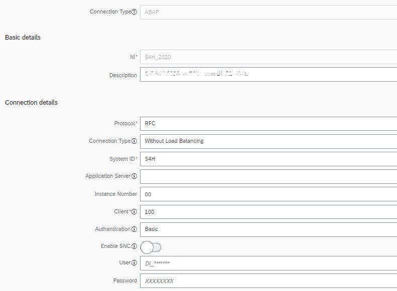

Note: In this case the SAP S/4HANA 2020 system has been equipped with all necessary Notes incl. the TCI 3105880.
Connection to Google Cloud Storage (GCS):

CDS view in the source SAP S/4HANA system:
The sample scenario in this blog will use an SAP S/4HANA system (on-premise) and a custom CDS view called “ZCDS_EPM_PO”, which has been created based on the EPM data model that comes with an SAP S/4HANA system. The CDS view is built based on table SEPM_BPA (Business Partners) and has the required Analytics annotations for data extraction + delta extraction as described here: https://help.sap.com/viewer/3a65df0ce7cd40d3a61225b7d3c86703/Cloud/en-US/55b2a17f987744cba62903e97dd...

More information about the EPM data model can be found here: https://help.sap.com/viewer/a602ff71a47c441bb3000504ec938fea/202009.latest/en-US/57e9f59831e94311852...
SAP Data Intelligence – Create and Execute a Generation 1 Graph
The design of the graph is quite simple and looks as follows:

Define CDS view extraction
Configure the CDS Reader Operator (here V2 is used) to extract data from CDS view “ZCDS_EPM_PO”.
- Connection: “S4H_2020”
- Version: ABAP CDS Reader V2
- Subscription type: New
- Subscription name: ZCDS_EPM_PO_01
- ABAP CDS Name: ZCDS_EPM_PO
- Transfer Mode: Replication
- Records per Roundtrip: 5000
- ABAP Data Type Conversion*: Enhanced Format Conversion (default)
* This parameter has been introduced recently, and its availability in the operator configuration panel depends on your SAP source system. If your system does not have the latest SAP Notes + TCI Note, this parameter might not be visible for you.

- Get CDS view columns
In a second step, a small Python operator is used to extract the CDS view columns out of the header provided in the output message of the CDS Reader operator to generate a CSV stream that contains the CDS view columns in the first row and the actual data body starting in the second line of the CSV data. Therefore, one input port of type message and one output port of type message are used.
There are various ways how to achieve this and you could, for example, pick the following example provided in a blog post by Yuliya Reich: https://blogs.sap.com/2021/02/15/sap-data-intelligence-how-to-get-headers-of-cds-view/. Note that the coding might need to be adjusted depending on your individual use case and the version of SAP S/4HANA you are using.
Code snippet based on Python 3.6:
from io import StringIO

import csv

import pandas as pd

import json


def on_input(inData):

    # read body

    data = StringIO(inData.body)


    # read attributes

    var = json.dumps(inData.attributes)

    result = json.loads(var)


    # from here we start json parsing

    ABAP = result['ABAP']

    Fields = ABAP['Fields']


    # creating an empty list for headers

    columns = []

    for item in Fields:

        columns.append(item['Name'])


    # data mapping using headers & saving into pandas dataframe

    df = pd.read_csv(data, index_col = False, names = columns)


    # here you can prepare your data,

    # e.g. columns selection or records filtering


    df_csv = df.to_csv(index = False, header = True)

    api.send('outString', df_csv)


api.set_port_callback('inData', on_input)- Write CSV file into Google Cloud Storage
As a last step the data needs to be loaded to Google Cloud Storage via CSV files. As a necessary prerequisite, the “to File” operator needs to be used as conversion operator to bring the data into the correct format that is required by the Write File operator.
In the Write File Operator configuration panel, we define the following parameters:
- Connection: GCS
- Path mode: Static with Placeholders
- Path: /demo/Generation1/ZCDS_EPM_PO/<date>/PO_<time>_<counter>.csv
- Mode: Create only
- If file exists: Fail
- Join Batches: False
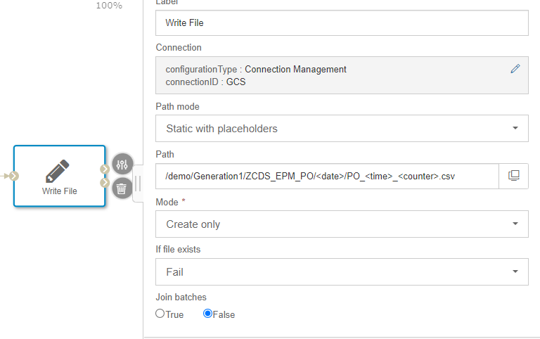
In this example file path “/demo/Generation1/ZCDS_EPM_PO/<date>/PO_<time>_<counter>.csv” is using different placeholder functions date, time and counter that will be generated during runtime of a graph whenever a data package is leaving the CDS Reader Operator and will be written into GCS. In this example each incoming data package will be stored and grouped in one folder of the current day, where each file name consists of the prefix “PO_” followed by the time of the data set arrival in the Write file operator and an integer counter that starts with 1 and will be enumerated by +1 for each data set streaming through the graph.
Example: /demo/Generation1/ZCDS_EPM_PO/20220103/PO_071053_1.csv
Please note that when you use the “Create Only” file mode that the placeholders in our example take care of writing all chunks of data into a dedicated file. When you use a plain graph without placeholders and only the first chunk of data will be written to GCS. Technically you can also make use of “Append” file mode, but depending on your scenario an “Append” creating large files might lead to memory problems when large files are created.
There are of course multiple other ways of designing the file name pattern that you can change based on your specific needs. You could for example create your own header information also in python and hand it over to the Write File operator as an input.
As we expect to run the graph 24x7 for initial load and change data capturing we do not add any graph terminator at the end of the graph.
When we now execute the graph, we will see that the following CSV files will be created in Google Cloud Storage as a target using the Metadata Explorer:
Once the initial load is done, there will be one file generated per incoming delta which occurred in the source. This can lead to smaller files being generated in case there is a low number of changes in your source system. Also here you can of course create mechanisms to merge batches into bigger chunks, but in this case, we want to keep it simple.
SAP Data Intelligence – Create and Execute a Generation 2 Graph:
Now we want to take the same use case we implemented with generation 1 operators to load data from a CDS view to CSV files in Google Cloud Storage and create a graph using the generation 2 operators. The high-level design of the generation 2 graph looks as follows:

1. Define CDS view extraction
In the first part we configure the Read Data from SAP System operator to extract data from CDS view “ZCDS_EPM_PO” using the following configuration parameters:
- Connection
The Connection of your SAP system created in the Connection Management containing all the necessary prerequisites mentioned in the beginning of this blog post. - Version
Select the version of the Read Data from SAP System operator. Please not that currently only one version is available of this operator. - Object Name
Browse and select the data set (in this case CDS view ZCDS_EPM_PO) you want to extract. Depending on your connected SAP system, you will either be able to browse within CDS folder (SAP S/4HANA Cloud or on premise) or within SLT folder (SAP Business Suite, SAP S/4HANA Foundation and SLT system).
- Transfer Mode
Choose between Initial Load, Replication and Delta Load transfer.
In our example scenario, we will select the following configurations:
- Select the connection to SAP S/4HANA, here “S4H_2020”
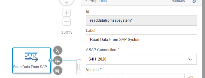
- Browse and select the Operator in “Version” parameter

- Browse the “Object” parameter to select “ZCDS_EPM_PO” CDS view:

Please note that you should not manually change the displayed value in the Object Name parameter once you selected your data set.
- Select Transfer Mode: “Replication”

2. Generate binary stream in CSV
Drag and drop the “Table to Binary” operator to the modelling canvas the and connect the output of the Read Data from SAP System operator to the input of the “Table to Binary” operator. The Table to Binary standard operator is required because the Binary Write File operator is requiring a binary input stream. It takes the table-based input from Read Data from SAP System operator and provides different capabilities in which format the data can be further processed, e.g. using CSV, JSON, JSON Lines or Parquet.In our case we select CSV as output format and the following CSV properties:

Note: The “colNames” parameter can be left empty as the column Names will automatically be extracted.

3. Write Partitioned CSV files to Google Cloud Storage
Drag and drop the generation 2 “Binary File Producer” to load the data via CSV files into Google Cloud Storage. Connect the output port “binary” of Table to Binary operator to the input port of the Binary File Producer operator.

In the Binary File Producer operator configuration panel, we define the following parameters:
- Connection ID: GCS
- Path mode: Static with Placeholders
- Path: /demo/Generation2/ZCDS_EPM_PO.csv
- Mode: Create only
- File mode: Partitioned File (required for using snapshots and resilience)
- Error Handling: terminate on error

In this example partitioned files File mode has been selected, which is a necessary prerequisite if we want to use graph resilience feature with snapshots with this operator. As file path parameter I have chosen: “/demo/Generation2/ZCDS_EPM_PO.csv”.
The main difference comparing the Generation 1 graph is that we now have a file mode parameter where we select “partitioned file mode”, which is required for using the snapshot feature. When partitioned file mode is selected, we can currently only define the path up to the partitioned file folder, in this example “ZCDS_EPM_PO.csv”, but not the actual file names of the various part files that are being generated inside our specified folder. The file name pattern is given and by using a generated uuid as well as the batch index that is included in the header information. More information about the handling of files including file name patterns can be checked here: https://help.sap.com/viewer/97fce0b6d93e490fadec7e7021e9016e/Cloud/en-US/64d01ad02e39499594b1eb10397...
There are of course multiple other ways of how you want to store your data in your file storage target system, e.g. using placeholders similar to generation 1 Write File operator in the file path, but in this case we want to keep it simple without using placeholders.
As we expect to run the graph 24x7 for initial load and change data capturing we do not use any graph terminator at the end of the graph.
Spoiler Alert: Usage of last batch and Graph Terminator in initial load mode
Using generation 2 Graphs and Operators there is also an improvement when e.g. using the Initial Load mode in the Read Data from SAP System operator which uses the “isLast” Batch attribute in the header, which is indicating whether the last chunk of data has been loaded from the SAP source system.
In the Graph Terminator operator there is a configuration parameter “On Last Batch”. If we change our graph to perform an “initial Load” in Transfer Mode parameter, add a graph Terminator after the Binary File Producer and set “on Last Batch” to True, the graph will automatically go to completed state when the load is completed:

Furthermore, you could also combine the usage of the Read Data from SAP System operator with structured data operators such as the Data Transform operator, e.g. for performing a projection on the CDS view, which was not possible using the generation 1 operators due to different port types being used by CDS Reader and Data Transform operators:
![]()
But now it’s time to execute our graph (using Replication Mode in the Read Data from SAP System operator) .
The way we execute the graph including the resiliency feature & snapshot is being done by clicking the “Run As” button in the Modeler:

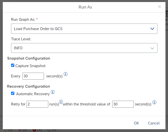
In the pop-up dialog, you can specify different options:
- Run Graph As: Specify the name of the graph execution that will be shown in the Modeler
e.g.: Load Purchase Order to Google Cloud Storage. - Snapshot Configuration: Enable
Every 30 seconds (default value)Note: Currently when using the Read Data from SAP System operator snapshots are mandatory and need to be enabled.
- Recovery Configuration: Enable
Retry for : “2” runs within the threshold value of “30” seconds.
Note: This parameter specifies whether the automatic restart feature should be used, which is optional. Whenever a graph is failing this feature will take care that the graph is restarted automatically with the maximum number of retries that are specified in “Retry for” within the time interval specified in the “threshold” parameter.
During the start time, you can check the Process Logs tab of your running graph and check out some new metrics that are provided by the generation 2 Read Data from SAP System operator, e.g.
- The completion rate of the access plan calculation in the source ABAP system (“calculation phase”)
- The completion rate of the initial load phase (“loading phase”)
- Begin of the replication / delta load phase
- Check the Work Process number as a reference to check it in the SAP ABAP backend system (“work process number”)

In addition, a new metric for the number of processed records has been introduced for the generation 2 Read Data from SAP System operator:

After the graph status is switching to “running” we can open the Metadata Explorer application to check the files being transferred to Google Cloud Storage.
When we browse inside the directory to the file path we defined “/demo/Generation2/ZCDS_EPM_PO.csv”, we will see that the following directory has been created:
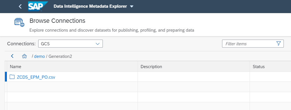
Inside the directory we can now see various part files that were replicated, where each part-file represents one batch of CDS view records. The generated part files follow the naming pattern
“part-<uuid>-<batch_index>.<file_extension>”,
e.g.: part-ffbc63eb-c582-4f90-b3c6-dbeb362e9977-0.csv

We can now also perform a quick data preview for one of the files to check the actual data that has been replicated from SAP S/4HANA to Google Cloud Storage:

Once the initial load is done, there will be one part file generated per incoming delta which occurred in the source. This can lead to smaller files being generated in case there are is a low change rate for the data in the source system. You can of course add mechanisms into your pipeline to merge batches into bigger chunks etc.
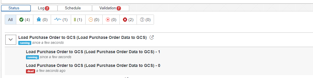
With our current configuration of snapshots and auto-restart, the graph will automatically re-start in case of an error and continue the replication using the snapshot information that has been captured at the point of failure.
In case an error happens, you will see in the lower section of the modeler that a new instance of the graph will be started and the failed one will still exist. Both executions are belonging and grouped together under the main graph we started:
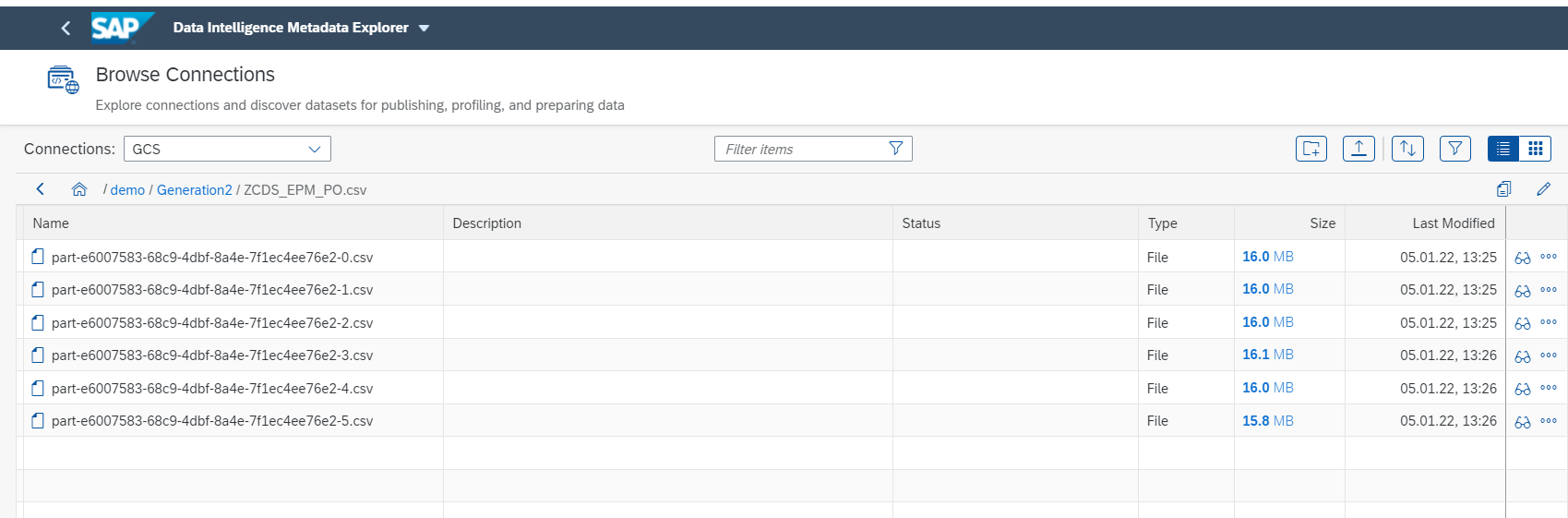
Before the error happens, we can see in the Metadata Explorer that up to batch index 5 the CSV files has been generated in Google Cloud Storage:
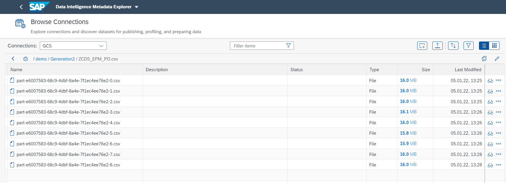
After the graph successfully restarts, we can see that the replication continues with batch index 6 to continue the replication:
In the overview section of your running or failed graph, you can also check the values you defined upon graph execution as well as the failure count etc.:

Conclusion
Now that’s it. I hope I could give you some useful information about the usage of ABAP integration with SAP Data Intelligence using Generation 2 graphs based on a sample scenario.
Please feel free to add your feedback and question in the comment section of this blog post.
- SAP Managed Tags:
- SAP Data Intelligence,
- ABAP Connectivity
Labels:
27 Comments
You must be a registered user to add a comment. If you've already registered, sign in. Otherwise, register and sign in.
Labels in this area
-
ABAP CDS Views - CDC (Change Data Capture)
2 -
AI
1 -
Analyze Workload Data
1 -
BTP
1 -
Business and IT Integration
2 -
Business application stu
1 -
Business Technology Platform
1 -
Business Trends
1,658 -
Business Trends
100 -
CAP
1 -
cf
1 -
Cloud Foundry
1 -
Confluent
1 -
Customer COE Basics and Fundamentals
1 -
Customer COE Latest and Greatest
3 -
Customer Data Browser app
1 -
Data Analysis Tool
1 -
data migration
1 -
data transfer
1 -
Datasphere
2 -
Event Information
1,400 -
Event Information
68 -
Expert
1 -
Expert Insights
177 -
Expert Insights
317 -
General
1 -
Google cloud
1 -
Google Next'24
1 -
GraphQL
1 -
Kafka
1 -
Life at SAP
780 -
Life at SAP
13 -
Migrate your Data App
1 -
MTA
1 -
Network Performance Analysis
1 -
NodeJS
1 -
PDF
1 -
POC
1 -
Product Updates
4,576 -
Product Updates
365 -
Replication Flow
1 -
REST API
1 -
RisewithSAP
1 -
SAP BTP
1 -
SAP BTP Cloud Foundry
1 -
SAP Cloud ALM
1 -
SAP Cloud Application Programming Model
1 -
SAP Datasphere
2 -
SAP S4HANA Cloud
1 -
SAP S4HANA Migration Cockpit
1 -
Technology Updates
6,873 -
Technology Updates
450 -
Workload Fluctuations
1
Related Content
- Second time a Leader in the Gartner® Magic Quadrant™ for Process Mining in Technology Blogs by SAP
- Understanding Data Modeling Tools in SAP in Technology Blogs by SAP
- Build Full Stack Applications in SAP BTP Cloud Foundry as Multi Target Applications (MTA) in Technology Blogs by Members
- The 2024 Developer Insights Survey: The Report in Technology Blogs by SAP
- Explore the SAP HANA Cloud vector engine with a free learning experience in Technology Blogs by SAP
Top kudoed authors
| User | Count |
|---|---|
| 21 | |
| 13 | |
| 11 | |
| 9 | |
| 8 | |
| 8 | |
| 7 | |
| 7 | |
| 6 | |
| 6 |