
- SAP Community
- Groups
- Interest Groups
- Application Development
- Blog Posts
- Safeguard Performance of ABAP CDS Views – Part 3 R...
Application Development Blog Posts
Learn and share on deeper, cross technology development topics such as integration and connectivity, automation, cloud extensibility, developing at scale, and security.
Turn on suggestions
Auto-suggest helps you quickly narrow down your search results by suggesting possible matches as you type.
Showing results for
former_member18
Active Participant
Options
- Subscribe to RSS Feed
- Mark as New
- Mark as Read
- Bookmark
- Subscribe
- Printer Friendly Page
- Report Inappropriate Content
12-20-2018
6:08 PM
In this blog post on the performance aspects of CDS views, I want to discuss how good performance can be ensured when building and accessing CDS views. Basically, it’s all about simple SQL performance rules that sometimes sink into oblivion when working with CDS views and HANA, but that are still valid - or only need a gentle new interpretation.
Here is the agenda of the blog series:
As we have seen in the previous blog posts, the hierarchy of CDS views and tables we build to reflect our data model turns into pure SQL when the CDS view is accessed from ABAP or HANA studio. Our intent – that is, which data we want to read – is declared in a single SQL string that gets processed by the SQL optimizer to create an execution plan.
So, before you start any work on CDS views, you should brush up your SQL know-how. This is especially important for us longtime ABAP developers, who previously often did not dare to implement ABAP Open SQL statements joining more than 3 tables. If you now embark on creating CDS views with dozens of underlying tables you should be aware of the complexity this can create, and you should have quite some SQL expertise to understand what it means to the database to process complex SQL statements.
A good starting point is to remember classical SQL performance rules like ‘avoid SQL statements in loops’ or ‘completely specify all known filter fields in the WHERE-clause’. Some of these rules are reflected for example in SAP’s 5 Golden Rules for database programming (see part 2 of ABAP on HANA – from analysis to optimization). From these rules I deduced what I think to be most relevant for implementing CDS views and SQL statements accessing these CDS views.
The less tables and views the database must join to process a request, the faster the statement preparation and plan creation, and often also the execution of the statement will be. The maintenance of a CDS view will be easier, and as we have seen in the previous blog post, also the created plans will be more stable for simple CDS views.
To a smaller extend, also the number of columns HANA needs to retrieve from the accessed tables in its column store, effects the runtime.
Therefore,
In the ABAP code snippet below there is an ABAP Open SQL join on CDS views I_BUSINESSUSER and I_PERSONWORKAGREEMENT, with 9 and 5 underlying tables, respectively. This join leads to a quite complex SQL statement. In fact, the author of the code just wanted to do an existence check for some USERID, which could be accomplished much simpler by joining two tables only. The author should talk to the owner(s) of the CDS views and ask whether they can provide a better-suited, slimmer CDS view.
HANA is very fast in searching entries in its column store. Joining very large tables, on the other hand, also takes its time on HANA. If you are joining several millions of entries from a header table with 10’s or 100’s of millions of entries in the associated line item table, and you are not applying any effective filter, don’t be surprised that response times will be in the many seconds range. Such a response time can be OK for a statement that is only rarely executed, maybe once or twice a day by a small group of users. The situation is totally different, if you expect a statement to be executed very frequently, by many users. Then, to keep system load low and user satisfaction high, you need to achieve response times in the (sub-)seconds range. If your statement is reading data from tables with very many (millions of) entries, effective filters to reduce the amount of to-be-processed data are a must.
To allow the filters to do their job, not only the WHERE-clauses should be given completely and contain selective fields, also in the join conditions all fields that define the table relationship should be specified. Otherwise it may happen that an existing filter field cannot be pushed to a joined branch of the SQL statement.
Specifying good filters is mandatory to achieve good performance on large data sets, but it is not enough. You should also check whether your filters really reach the underlying tables. To this end, executing performance tests with reasonable (that is, production-like) test data and analyzing SQL traces and HANA execution plans with the HANA PlanViz tool are a must. In the plan, we need to keep an eye on intermediate results.
Intermediate results are the ‘output’ of the plan operators, for example of filters, joins, or aggregations. The strategy of the SQL optimizer is to reduce intermediate results in plan execution as early as possible, and as effective as possible. Or: the faster the size of result sets can be reduced, the less will be the effort for subsequent processing steps. You already know the best way to support the SQL optimizer with this task: provide effective filters that can be pushed down towards the data source.
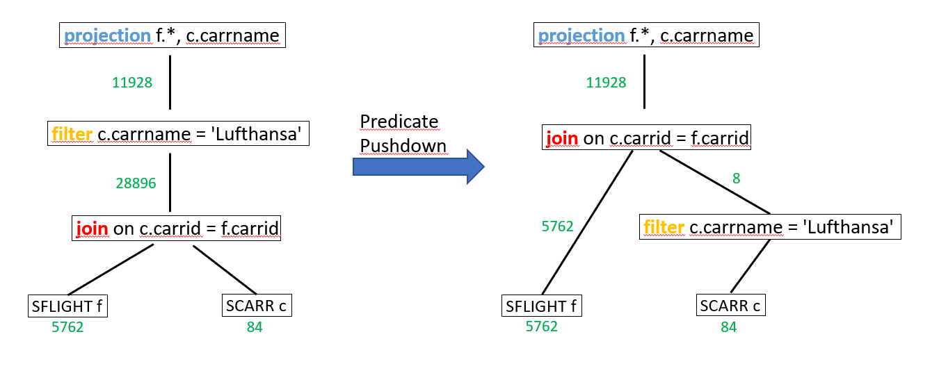
In the picture below, we see the optimization for this SQL statement:
The join between SFLIGHT and SCARR would have an intermediate result of 28.896 rows (left side). When the filter is pushed down to table SCARR (‘Predicate Pushdown’, right side), the intermediate result of the join is only 11.928 rows. So, by applying the filter early in the plan processing, the size of intermediate results could be reduced drastically.
While the intermediate results of some operators (e.g. filters, some sort of joins) can be administrated quite efficiently inside the column engine, other operators need to ‘see’ the whole intermediate result to proceed with their work.
This leads to ‘materialized’ intermediate results, which means that in-memory copies of the result must be created as temporary internal tables on HANA. If the materialized results are large, they have a significant impact on the performance of SQL statement execution.
In the HANA PlanViz tool, large intermediate results can be identified by high numbers shown besides the connection lines of two operator boxes. In the screen shot from PlanViz below, intermediate results have been materialized due to a calculated field used in a join condition. More than 9 million entries must be copied, leading to a runtime of more than 2 seconds for a simple SQL statement.

As a rule of thumb, if millions of entries are passed between operators, runtimes in the many-seconds range must be expected. Besides that, big materialized intermediate results can also lead to out-of-memory situations on HANA.
Materialized intermediate results are caused by:
One of the main reasons for materialization are calculated fields. These – with the special case of ‘not NULL-preserving’ fields – will be discussed now.
A simple case of a calculated field is a field concatenated from other fields of the same table or view. Look at this view definition:
If this CDS view is accessed via it’s concatenated key,
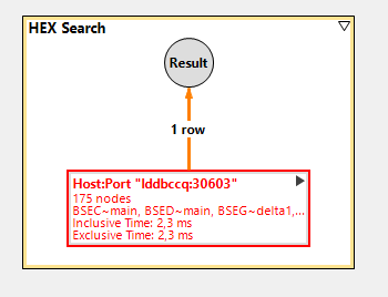
this takes more than 2 seconds in one of our performance tests systems. The reason is, that for more than 9 million entries in table BSEG, the concatenated key must be calculated before the filter can be applied. See the screen shot from PlanViz tool:

Fortunately, this CDS view also contains the single fields of the concatenated key (that is, there is some redundancy), so one can also access the view this way:
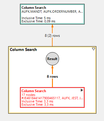
The execution of this statement just takes 2,3 ms. In my performance test system, the statement is already processed by the new HANA processing engine:
If our example view would be frequently accessed using only the calculated field ChangeDocumentTableKey as filter, it could be a good idea to persist this field in the view instead of calculating it for all rows in every access. Alternatively, an additional materialized (here: persisted) view for mapping the calculated field to a new, proper CDS key of the main view could be created. Both solutions are a trade-off between additional memory consumption due to the additional field or view against improved execution runtime for the access.
Fields that result from string operations like CONCAT, RTRIM or SUBSTRING, from functions like COALESCE, or from numeric calculations are called calculated fields. Also, fields that are defined within a CASE ... WHEN … ELSE construct are calculated fields.
These kinds of fields can lead to problems when the following conditions are met:
When field ‘fldR’ is not NULL-preserving, the SQL optimizer cannot swap the execution order of LEFT OUTER JOIN and calculation. Therefore, it is necessary to build up a materialization of View_R, and fldR is calculated for every row in View_R, even for those that are discarded after the join.
The following illustration depicts why a permutation of the join and the not NULL-preserving result leads to different results


Let’s look at an example for the impact of a not NULL-preserving field. I created a simple CDS view “cds_1” that joins table AUFK (order master data) with another CDS view “cds_2” with a LEFT OUTER JOIN. In view “cds_2”, there is a LEFT OUTER JOIN between the tables JEST (object status) and JSTO (status object information).

With the option ‘Show SQL Create Statement’ in ADT it is possible to get an SQL representation of a CDS view. Together with the SQL statement accessing the view I get this statement:
As you see, I inserted a not NULL-preserving ELSE ‘X’ into the SQL statement, more precisely into the inner CDS view. The execution of the SQL statement in one of our performance test systems takes 6 seconds and has the following result and PlanViz trace:


In the plan, we recognize both a high number of rows that are copied between the operator boxes (nearly 13 million) and the 'stacked column search' operators. The latter are a sign that not all filters could be pushed down. The database had to materialize all rows of table JEST to fill the field ISUSERSTATUS before the filter could be applied.
In a customer system with much more entries in table JEST, the runtime of this statement could easily achieve one minute.
One way to improve the situation is to move the CASE … ELSE branch one level higher, that is 'after' the first join. The statement then looks like this:
The runtime for this statement is down to 5 ms. The filter can be applied early and the calculation needs to be executed only on the small filtered result set (8 entries).
Another way to improve the SQL statement / CDS view would be to eliminate the ELSE-branch entirely. This is possible, if the consumer of the statement can live with NULL values in the result set.


The runtime of this statement is also around 5 ms.
Some recommendations for calculated fields including not NULL-preserving fields:
For CASE ... ELSE statements:
This is the 5th of the Golden Rules for database programming and it seems to be the most outdated in times of HANA and mottoes like ‘move data-intensive calculations to the database’. But still, striving for minimal resource consumption is key also for the database. Unnecessary database accesses and calculations must be avoided, and as one example, the good old buffering of tables or CDS views on the ABAP application server is still possible and recommended.
Furthermore, new caches have been introduced on the HANA server for aggregated data. Imagine when in the morning hundreds of users log in to a system to display some Fiori Overview Page. It does not make sense to calculate identical key figures on these pages again and again for every user. Instead, the data could as well be read from HANA’s static result cache. Beside this, a dynamic result cache is developed, and both application specific caches and aggregate tables still have their justification.
Here is the agenda of the blog series:
- Part 1 – CDS View Complexity
- Part 2 – HANA SQL Optimizer and Plan Cache
- Part 3 – Rules for Good Performance of CDS Views - this blog
- Part 4 – Data Modelling
- Part x – maybe more … your ideas or questions
Fresh up your SQL
As we have seen in the previous blog posts, the hierarchy of CDS views and tables we build to reflect our data model turns into pure SQL when the CDS view is accessed from ABAP or HANA studio. Our intent – that is, which data we want to read – is declared in a single SQL string that gets processed by the SQL optimizer to create an execution plan.
So, before you start any work on CDS views, you should brush up your SQL know-how. This is especially important for us longtime ABAP developers, who previously often did not dare to implement ABAP Open SQL statements joining more than 3 tables. If you now embark on creating CDS views with dozens of underlying tables you should be aware of the complexity this can create, and you should have quite some SQL expertise to understand what it means to the database to process complex SQL statements.
A good starting point is to remember classical SQL performance rules like ‘avoid SQL statements in loops’ or ‘completely specify all known filter fields in the WHERE-clause’. Some of these rules are reflected for example in SAP’s 5 Golden Rules for database programming (see part 2 of ABAP on HANA – from analysis to optimization). From these rules I deduced what I think to be most relevant for implementing CDS views and SQL statements accessing these CDS views.
Minimize the number of accessed objects, operations, and table columns
The less tables and views the database must join to process a request, the faster the statement preparation and plan creation, and often also the execution of the statement will be. The maintenance of a CDS view will be easier, and as we have seen in the previous blog post, also the created plans will be more stable for simple CDS views.
To a smaller extend, also the number of columns HANA needs to retrieve from the accessed tables in its column store, effects the runtime.
Therefore,
- In your CDS views, expose only required fields to reduce the number of accessed tables, used joins and operations
- Use associations instead of LEFT OUTER JOINs, so that additional joins are only executed when fields from associations are explicitly requested by path notation
- If possible, define outer joins as LEFT OUTER MANY TO ONE joins and associations with “TO ONE” cardinality ([n..1]). In this case, if no field is requested from the joined table, the database can avoid executing the join at runtime.
Note that a wrongly stated “TO ONE” cardinality can lead to functional errors, if true the cardinality would be “TO MANY”. - In the SQL statement accessing the CDS view, only request those fields required for your application. A SELECT * statement requires that many columns are accessed, which creates some costs for the HANA column store. You should prefer to use a well-defined field list instead. But please note, that several accesses to the same table / view with varying field lists are not worth-while. It is more effective to have only one database access requiring all fields needed for processing the application.
- Also using lengthy GROUP BY clauses make it necessary to access many columns. Generally, try to avoid GROUP BY clauses in CDS views that are re-used in a CDS view hierarchy.
- Data modelling tips will follow in next blog post. For the moment note, that any CDS view should be well-suited to the business requirements it has to fulfill and should not contain superfluous tables. Reuse of CDS views must not be exaggerated in a way that for an application there is only one or a handful of one-size-fits-all views that can do almost everything (that is, answer all possible queries).
In the ABAP code snippet below there is an ABAP Open SQL join on CDS views I_BUSINESSUSER and I_PERSONWORKAGREEMENT, with 9 and 5 underlying tables, respectively. This join leads to a quite complex SQL statement. In fact, the author of the code just wanted to do an existence check for some USERID, which could be accomplished much simpler by joining two tables only. The author should talk to the owner(s) of the CDS views and ask whether they can provide a better-suited, slimmer CDS view.
SELECT a~userid FROM i_businessuser WITH PRIVILEGED ACCESS AS a

    INNER JOIN i_personworkagreement WITH PRIVILEGED ACCESS AS b

           ON    a~businesspartner = b~person

           WHERE b~personworkagreement = @ls_approver-objid INTO @DATA(lv_userid) UP TO 1 ROWS.

ENDSELECT.
Apply selective filters - and check that they reach their target
HANA is very fast in searching entries in its column store. Joining very large tables, on the other hand, also takes its time on HANA. If you are joining several millions of entries from a header table with 10’s or 100’s of millions of entries in the associated line item table, and you are not applying any effective filter, don’t be surprised that response times will be in the many seconds range. Such a response time can be OK for a statement that is only rarely executed, maybe once or twice a day by a small group of users. The situation is totally different, if you expect a statement to be executed very frequently, by many users. Then, to keep system load low and user satisfaction high, you need to achieve response times in the (sub-)seconds range. If your statement is reading data from tables with very many (millions of) entries, effective filters to reduce the amount of to-be-processed data are a must.
Filter rules
- Filters can be set via WHERE-clauses in CDS views
- Filters are always propagated through projections
- Filters are propagated through joins only via fields in ON-condition
- Filters are not pushed through calculations (functions) – see below
To allow the filters to do their job, not only the WHERE-clauses should be given completely and contain selective fields, also in the join conditions all fields that define the table relationship should be specified. Otherwise it may happen that an existing filter field cannot be pushed to a joined branch of the SQL statement.
Different from what you might expect, the LIMIT option (UP TO n ROWS or SELECT SINGLE in ABAP Open SQL) is no replacement for a good filter. The LIMIT is most often applied very late in the SQL processing, after all the expensive operations like joins and calculations have been executed on the full data set. The reason is that a lot of operations (ORDER BY, DISTINCT, aggregations, cardinality changing joins) prohibit an early application of a limit.
Specifying good filters is mandatory to achieve good performance on large data sets, but it is not enough. You should also check whether your filters really reach the underlying tables. To this end, executing performance tests with reasonable (that is, production-like) test data and analyzing SQL traces and HANA execution plans with the HANA PlanViz tool are a must. In the plan, we need to keep an eye on intermediate results.
Intermediate Results
Intermediate results are the ‘output’ of the plan operators, for example of filters, joins, or aggregations. The strategy of the SQL optimizer is to reduce intermediate results in plan execution as early as possible, and as effective as possible. Or: the faster the size of result sets can be reduced, the less will be the effort for subsequent processing steps. You already know the best way to support the SQL optimizer with this task: provide effective filters that can be pushed down towards the data source.
In the picture below, we see the optimization for this SQL statement:
SELECT f.*, c.carrname

   FROM SFLIGHT AS f

   INNER JOIN SCARR AS c

   ON c.carrid = f.carrid

WHERE c.carrname = 'Lufthansa'
The join between SFLIGHT and SCARR would have an intermediate result of 28.896 rows (left side). When the filter is pushed down to table SCARR (‘Predicate Pushdown’, right side), the intermediate result of the join is only 11.928 rows. So, by applying the filter early in the plan processing, the size of intermediate results could be reduced drastically.
Materialized Results
While the intermediate results of some operators (e.g. filters, some sort of joins) can be administrated quite efficiently inside the column engine, other operators need to ‘see’ the whole intermediate result to proceed with their work.
This leads to ‘materialized’ intermediate results, which means that in-memory copies of the result must be created as temporary internal tables on HANA. If the materialized results are large, they have a significant impact on the performance of SQL statement execution.
In the HANA PlanViz tool, large intermediate results can be identified by high numbers shown besides the connection lines of two operator boxes. In the screen shot from PlanViz below, intermediate results have been materialized due to a calculated field used in a join condition. More than 9 million entries must be copied, leading to a runtime of more than 2 seconds for a simple SQL statement.
As a rule of thumb, if millions of entries are passed between operators, runtimes in the many-seconds range must be expected. Besides that, big materialized intermediate results can also lead to out-of-memory situations on HANA.
Materialized intermediate results are caused by:
- Operations that must switch the HANA engine for execution, for example from column engine to row engine:
- Operations on cyclic joins
- Non-equi joins
- Window functions
In future, HANA will significantly reduce engine switches with enhanced state-of-the-art query processing features.
- Frustrated join push-down (switch of join and calculation operators is not possible). As a symptom one finds stacked column search operations in the execution plan (as in the screen shot above). Reasons are:
- Filter / join on calculated fields
- Not NULL-preserving calculations
- Constants in join conditions
One of the main reasons for materialization are calculated fields. These – with the special case of ‘not NULL-preserving’ fields – will be discussed now.
Calculated Fields
A simple case of a calculated field is a field concatenated from other fields of the same table or view. Look at this view definition:
define view I_WithCalculatedField

  as select from bseg as AccountingDocSeg

{

  key concat(mandt,

          concat(bukrs,

              concat(belnr,

                  concat(gjahr, buzei)

              )

          )

      )                                         as ChangeDocumentTableKey,

  key cast('BSEG' as farp_database_table_name ) as DatabaseTable,

  key buzei                                      as AccountingDocumentItem,

      cast( belnr as farp_belnr_d )              as AccountingDocument,

      bukrs                                      as CompanyCode,

      gjahr                                      as FiscalYear,

      hkont                                      as GLAccount,

      kunnr                                      as Customer,

      lifnr                                      as Supplier,

      bschl                                      as PostingKey,

      koart                                      as AccountType,

      umskz                                      as SpecialGLCode

}
If this CDS view is accessed via it’s concatenated key,
select * from IWthCalcFld where mandt = '910' and

            ChangeDocumentTableKey = '910000149001109892018002'
this takes more than 2 seconds in one of our performance tests systems. The reason is, that for more than 9 million entries in table BSEG, the concatenated key must be calculated before the filter can be applied. See the screen shot from PlanViz tool:
Fortunately, this CDS view also contains the single fields of the concatenated key (that is, there is some redundancy), so one can also access the view this way:
select * from IWthCalcFld where mandt = '910' and

               companycode = '0001' and

               AccountingDocument = '4900110989' and

               FiscalYear = '2018' and

               AccountingDocumentItem = '002'
The execution of this statement just takes 2,3 ms. In my performance test system, the statement is already processed by the new HANA processing engine:
If our example view would be frequently accessed using only the calculated field ChangeDocumentTableKey as filter, it could be a good idea to persist this field in the view instead of calculating it for all rows in every access. Alternatively, an additional materialized (here: persisted) view for mapping the calculated field to a new, proper CDS key of the main view could be created. Both solutions are a trade-off between additional memory consumption due to the additional field or view against improved execution runtime for the access.
Fields that result from string operations like CONCAT, RTRIM or SUBSTRING, from functions like COALESCE, or from numeric calculations are called calculated fields. Also, fields that are defined within a CASE ... WHEN … ELSE construct are calculated fields.
Not NULL-preserving calculated fields
These kinds of fields can lead to problems when the following conditions are met:
- A CDS view ‘View_R’ contains a ‘not NULL-preserving’ calculated field ‘fldR’. A calculation is not NULL-preserving, if the calculation result cannot be NULL even if the input value is NULL.
Examples are the COALESCE( arg1, arg 2) statement and the CASE statement:
case
when attr1 like 'E%' then 'X'
else ' '
end as fldR,
// the value of fldR will never be NULL, regardless of input
- In the next level view ‘View_T’, View_R is joined via LEFT OUTER JOIN to a table or view ‘View_L’, being the right side of the join AND the field ‘fldR’ is exposed in ‘View_T’
When field ‘fldR’ is not NULL-preserving, the SQL optimizer cannot swap the execution order of LEFT OUTER JOIN and calculation. Therefore, it is necessary to build up a materialization of View_R, and fldR is calculated for every row in View_R, even for those that are discarded after the join.
The following illustration depicts why a permutation of the join and the not NULL-preserving result leads to different results
Let’s look at an example for the impact of a not NULL-preserving field. I created a simple CDS view “cds_1” that joins table AUFK (order master data) with another CDS view “cds_2” with a LEFT OUTER JOIN. In view “cds_2”, there is a LEFT OUTER JOIN between the tables JEST (object status) and JSTO (status object information).
With the option ‘Show SQL Create Statement’ in ADT it is possible to get an SQL representation of a CDS view. Together with the SQL statement accessing the view I get this statement:
SELECT * FROM

 ( SELECT

 "AUFK"."MANDT" AS "MANDT",

 "AUFK"."AUFNR" AS "ORDERNUMBER",

 "AUFK"."OBJNR" AS "OBJECTNUMBER",

 "STATUS"."ISUSERSTATUS" AS "ISUSERSTATUS"

FROM "AUFK" "AUFK"

LEFT OUTER JOIN (

SELECT

 "JEST"."MANDT" AS "MANDT",

 "JSTO"."OBJNR" AS "STATUSOBJECT",

 "JEST"."STAT" AS "STATUSCODE",

CASE "JEST"."STAT"

  WHEN 'I0001' THEN "JEST"."STAT"

  WHEN 'I0002' THEN "JEST"."STAT"

  WHEN 'I0115' THEN "JEST"."STAT"

  ELSE 'X'                -- <<<<<<<<<<<<<<<<<<

      END AS "ISUSERSTATUS",

 "JEST"."INACT" AS "STATUSISINACTIVE"

FROM "JEST" "JEST"

LEFT OUTER JOIN "JSTO" "JSTO"

ON ( "JEST"."MANDT" = "JSTO"."MANDT"

AND "JEST"."OBJNR" = "JSTO"."OBJNR" )

WHERE ( "JEST"."MANDT" = SESSION_CONTEXT( 'CDS_CLIENT' ) ) ) "STATUS"

ON ( "AUFK"."MANDT" = "STATUS"."MANDT"

AND "AUFK"."OBJNR" = "STATUS"."STATUSOBJECT" )

WHERE ( "AUFK"."MANDT" = SESSION_CONTEXT( 'CDS_CLIENT' ) ) )

WHERE "MANDT" = '800'

AND "ORDERNUMBER" = '000004001784'
As you see, I inserted a not NULL-preserving ELSE ‘X’ into the SQL statement, more precisely into the inner CDS view. The execution of the SQL statement in one of our performance test systems takes 6 seconds and has the following result and PlanViz trace:
In the plan, we recognize both a high number of rows that are copied between the operator boxes (nearly 13 million) and the 'stacked column search' operators. The latter are a sign that not all filters could be pushed down. The database had to materialize all rows of table JEST to fill the field ISUSERSTATUS before the filter could be applied.
In a customer system with much more entries in table JEST, the runtime of this statement could easily achieve one minute.
One way to improve the situation is to move the CASE … ELSE branch one level higher, that is 'after' the first join. The statement then looks like this:
SELECT * FROM ( SELECT

 "AUFK"."MANDT" AS "MANDT",

 "AUFK"."AUFNR" AS "ORDERNUMBER",

 "AUFK"."OBJNR" AS "OBJECTNUMBER",

 CASE "ISUSERSTATUS"

 WHEN 'I0001' THEN "ISUSERSTATUS"

 WHEN 'I0002' THEN "ISUSERSTATUS"

 WHEN 'I0115' THEN "ISUSERSTATUS"

ELSE 'X'                 -- <<<<<<<<<<<<<<<<<

END AS "ISUSERSTATUS"

FROM "AUFK" "AUFK"

LEFT OUTER JOIN ( SELECT

 "JEST"."MANDT" AS "MANDT",

 "JSTO"."OBJNR" AS "STATUSOBJECT",

 "JEST"."STAT" AS "STATUSCODE",

     "JEST"."STAT" as "ISUSERSTATUS",

 "JEST"."INACT" AS "STATUSISINACTIVE"

FROM "JEST" "JEST"

LEFT OUTER JOIN "JSTO" "JSTO" ON ( "JEST"."MANDT" = "JSTO"."MANDT"

AND "JEST"."OBJNR" = "JSTO"."OBJNR" )

WHERE ( "JEST"."MANDT" = SESSION_CONTEXT( 'CDS_CLIENT' ) ) ) "STATUS" ON ( "AUFK"."MANDT" = "STATUS"."MANDT"

AND "AUFK"."OBJNR" = "STATUS"."STATUSOBJECT" )

WHERE ( "AUFK"."MANDT" = SESSION_CONTEXT( 'CDS_CLIENT' ) ) )

WHERE "MANDT" = '800'

AND "ORDERNUMBER" = N'000004001784' WITH RANGE_RESTRICTION( 'CURRENT')
The runtime for this statement is down to 5 ms. The filter can be applied early and the calculation needs to be executed only on the small filtered result set (8 entries).
Another way to improve the SQL statement / CDS view would be to eliminate the ELSE-branch entirely. This is possible, if the consumer of the statement can live with NULL values in the result set.
The runtime of this statement is also around 5 ms.
Some recommendations for calculated fields including not NULL-preserving fields:
- Calculated fields should be avoided in views that might be associated from other views or are known to be used on the right side of a left outer join
- Calculations should best be done in the consumption view (highest level view), after all filters and data reducing joins have already happened. This might require a complex re-work of the whole view hierarchy.
- Interface views shall not define calculated fields.
- Calculated fields should not be used as main filter field – filters cannot be pushed down through calculations
- Calculated fields should be avoided in join conditions
- To avoid calculations and enable filter push-down, introducing redundancy and / or persisting a calculated field in the table is a valid option.
For CASE ... ELSE statements:
- Constants shall not be used in the ELSE-clause of a CASE statement
- The ELSE-clause in the CASE statement should be omitted, unless it is necessary (even if development tools recommend otherwise …)
Keep unnecessary load away from the database
This is the 5th of the Golden Rules for database programming and it seems to be the most outdated in times of HANA and mottoes like ‘move data-intensive calculations to the database’. But still, striving for minimal resource consumption is key also for the database. Unnecessary database accesses and calculations must be avoided, and as one example, the good old buffering of tables or CDS views on the ABAP application server is still possible and recommended.
Furthermore, new caches have been introduced on the HANA server for aggregated data. Imagine when in the morning hundreds of users log in to a system to display some Fiori Overview Page. It does not make sense to calculate identical key figures on these pages again and again for every user. Instead, the data could as well be read from HANA’s static result cache. Beside this, a dynamic result cache is developed, and both application specific caches and aggregate tables still have their justification.
- SAP Managed Tags:
- ABAP Development
11 Comments
You must be a registered user to add a comment. If you've already registered, sign in. Otherwise, register and sign in.
Labels in this area
-
A Dynamic Memory Allocation Tool
1 -
ABAP
10 -
ABAP 7.4
1 -
abap cds
1 -
ABAP CDS Views
14 -
ABAP class
1 -
ABAP Cloud
1 -
ABAP Development
5 -
ABAP in Eclipse
2 -
ABAP Keyword Documentation
2 -
ABAP OOABAP
3 -
ABAP Programming
1 -
abap technical
1 -
ABAP test cockpit
7 -
ABAP test cokpit
1 -
Adobe Form
1 -
ADT
1 -
Advanced Event Mesh
1 -
AEM
1 -
AI
1 -
ALV
1 -
alv oo
1 -
API and Integration
1 -
APIs
9 -
APIs ABAP
1 -
App Dev and Integration
1 -
Application Development
2 -
application job
1 -
archivelinks
1 -
Automation
4 -
B2B Integration
1 -
BTP
1 -
CAP
1 -
CAPM
1 -
Career Development
3 -
CL_GUI_FRONTEND_SERVICES
1 -
CL_SALV_TABLE
2 -
Cloud Extensibility
8 -
Cloud Native
7 -
Cloud Platform Integration
1 -
CloudEvents
2 -
CMIS
1 -
Connection
1 -
container
1 -
Customer Portal
1 -
Debugging
2 -
Developer extensibility
1 -
Developing at Scale
3 -
DMS
1 -
dynamic logpoints
1 -
Dynpro
1 -
Dynpro Width
1 -
Eclipse ADT ABAP Development Tools
1 -
EDA
1 -
Event Mesh
1 -
Expert
1 -
Field Symbols in ABAP
1 -
Fiori
1 -
Fiori App Extension
1 -
Forms & Templates
1 -
General
1 -
Getting Started
1 -
IBM watsonx
2 -
Integration & Connectivity
10 -
Introduction
1 -
JavaScripts used by Adobe Forms
1 -
joule
1 -
NodeJS
1 -
ODATA
3 -
OOABAP
4 -
Outbound queue
1 -
ProCustomer
1 -
Product Updates
1 -
Programming Models
14 -
Restful webservices Using POST MAN
1 -
RFC
1 -
RFFOEDI1
1 -
SAP BAS
1 -
SAP BTP
1 -
SAP Build
1 -
SAP Build apps
1 -
SAP Build CodeJam
1 -
SAP CodeTalk
1 -
SAP Odata
2 -
SAP SEGW
1 -
SAP UI5
1 -
SAP UI5 Custom Library
1 -
SAPEnhancements
1 -
SapMachine
1 -
security
3 -
SM30
1 -
Table Maintenance Generator
1 -
text editor
1 -
Tools
18 -
translation
1 -
User Experience
6 -
Width
1
Top kudoed authors
| User | Count |
|---|---|
| 4 | |
| 3 | |
| 3 | |
| 2 | |
| 2 | |
| 2 | |
| 1 | |
| 1 | |
| 1 | |
| 1 |