- SAP Community
- Products and Technology
- Human Capital Management
- HCM Blogs by SAP
- Creation of a flexible Headcount Time Series with ...
- Subscribe to RSS Feed
- Mark as New
- Mark as Read
- Bookmark
- Subscribe
- Printer Friendly Page
- Report Inappropriate Content
Introduction
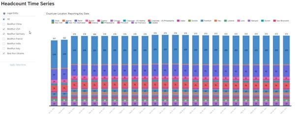
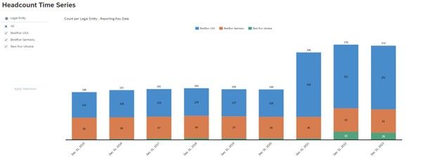
The Employee Central (EC) data model follows the guiding principle of “effective-dated” time slices. This means any change of the employment (or other entities as e.g. personal data, compensation data or others) generates a new effective dated time slice, which could be any date. Even multiple changes per day are possible for various EC entities. However, the reporting of a time series requires the data transformation into well-defined time slices as e.g. the determination of the employment situation of all employees to particular reporting key dates. Typically, such reporting key dates would then be the month end dates (as shown in Figure 1 below) or e.g. the last day of each year (as shown in Figure 2 below). The approach used in the blog post is a kind of trick to fold the arbitrarily distributed time slice lengths with a clearly defined time grid.
Figure 1 – Monthly time series of the headcount visualized with a Stacked Bar chart which uses the dimension Location
Figure 2 – Yearly time series of the headcount visualized with a Stacked Bar chart which uses the dimension Legal Entity
In the following the technical design (1) of the configuration entities and (2) of the data source and of the story is described.
Technical design of the configuration entities
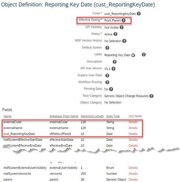
First, it is required to create a MDF object for the Reporting Key Dates; the object which is shown in Figure 3 is called cust_ReportingKeyDate. See the attributes of this object indicated in Figure 3. Important is to define “Effective Dating = From Parent” and to define cust_RepotingKeyDate of Data Type “Date” (it’s recommended to switch visibility of externalName to ‘Not Visible’).
Figure 3 Definition of custom MDF object cust_ReportingKeyDate
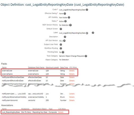
Afterwards, it is required to create another custom MDF object cust_LegalEntityReportingKeyDate with the attributes as indicated in Figure 4. Import is to define an Association of type “Composite”, Multiplicity “One To Many” to the previously created custom MDF object “Reporting Key Date” as ‘Destination Object” (also here it is recommended to switch visibility of externalName to ‘Not Visible’).
Figure 4 Definition of custom MDF object cust_LegalEntityReportingKeyDate
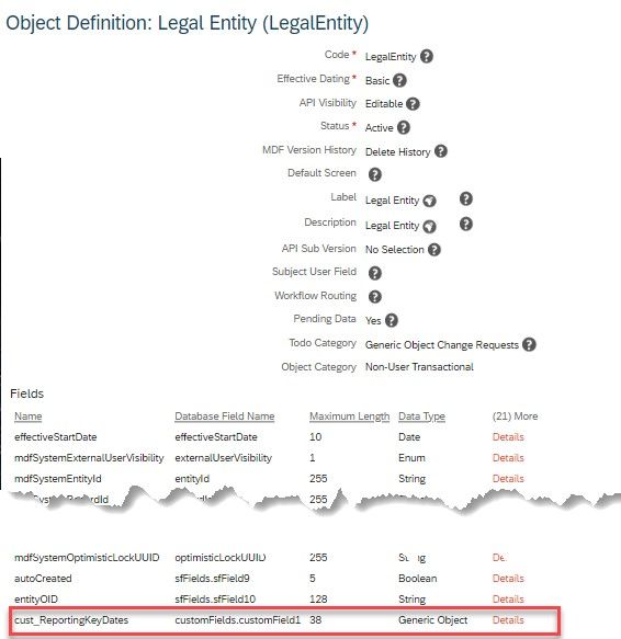
As 3rd and last step it is required to add a custom field ‘cust_ReportingKeyDates’ to the MDF object “Legal Entity”. Use Data Type “cust_LegalEntityReportingKeyDate” and Label “Reporting Key Dates” as indicated in Figure 5.
Figure 5 Custom field cust_LegalEntityReportingKeyDate added to MDF object Legal Entity
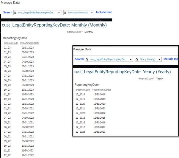
Now it is possible to maintain “Reporting Key Dates” at custom MDF object cust_LegalEntityReportingKeyDate as indicated at Figure 6. Figure 6 shows the Reporting Key Dates for a monthly time series (left) and a yearly time series (right). Of course, it’s possible also to maintain additional instances for this MDF object to generate e.g., weekly or quarterly time series.
Figure 6 Maintenance of Reporting Key Dates at custom MDF object cust_LegalEntityReportingKeyDate
The 2nd maintenance step is to assign the previously created entities for cust_LegalEntityReportingKeyDate (in Figure 6 called “Monthly” and “Yearly”) to the Legal Entity.
Finally, navigate to "Manage Data" => "Report Object Configuration Entity" and edit both newly created objects and maintain "Employment" as "Sub-Domain Schema List". This guarantees that both objects are available as navigation targets under schema "Employment" in the query designer.
Technical design of the data source
The data source for the creation of the time series is indicated at Figure 7. Note that there is no time filter applied to “Job Information” and time filter = “Today” is applied to “Legal Entity”.
Figure 7 Query to generate the time series
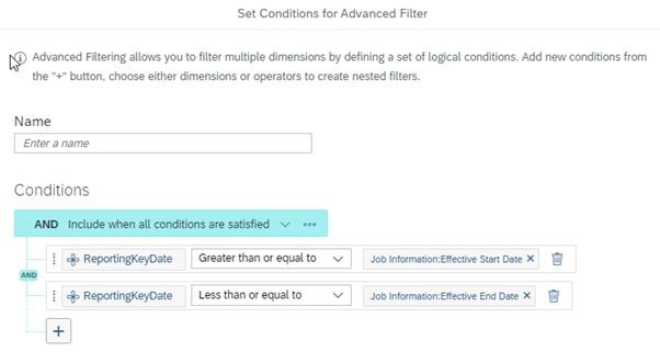
Finally, it is required to apply a filter to pick up the correct combination of “Job information” time slice and the record of “Reporting Key Date”. To illustrate this necessity, think about following example: Assume the job information history has 5 effective-dated time slice and “Reporting Key Date” has 36 records (= monthly reporting key dates of the last 3 years). Then the query would provide 180 (=5 x 36) records. The filter indicated at Figure 8 takes care that only the relevant record for the reporting key date is picked up from Job Information. After the filtering, the query would provide 36 records per employee.
Figure 8 Filter condition to pick up the relevant job information record
Now it is possible to create a chart based on this query. The charts from Figure 1 and 2 are of chart type “Stacked Bar/Column” (with Measure “Count”, Dimension “Reporting Key Date” and usage of dimension “Location” (Figure 1) and “Legal Entity” (Figure 2) under “Color”). It is important to apply a filter for “Employment Status” as ‘Active’, Unpaid Leave’ ‘Paid Leave’ and ‘Suspended’ so that only “Active” employees are reported (maybe other values for employment status are relevant for your reporting use case).
Of course, the charts indicated at Figure 1 and 2 are just examples. It is possible to use other chart types (e.g. “Time Series”), other measures (e.g. FTE instead of ‘Count’), other dimensions (e.g. pay grade, gender, age ranges instead of location and legal entity) and other time range grid steps (e.g. quarterly, bi-weekly, etc.).
- SAP Managed Tags:
- SAP SuccessFactors People Analytics,
- SAP SuccessFactors Workforce Analytics
You must be a registered user to add a comment. If you've already registered, sign in. Otherwise, register and sign in.
-
1H 2023 Product Release
3 -
2H 2023 Product Release
3 -
Business Trends
104 -
Business Trends
4 -
Cross-Products
13 -
Event Information
75 -
Event Information
8 -
Events
5 -
Expert Insights
26 -
Expert Insights
21 -
Feature Highlights
16 -
Hot Topics
20 -
Innovation Alert
8 -
Leadership Insights
4 -
Life at SAP
67 -
Life at SAP
1 -
Product Advisory
5 -
Product Updates
499 -
Product Updates
44 -
Release
6 -
Technology Updates
408 -
Technology Updates
13
- How to create measure based input control in successfactors people analytics stories in Human Capital Management Q&A
- A Deep Dive into Tacking New Hires and Leavers Trends - How to build monthly trending reports by using story report tool in SuccessFactors in Human Capital Management Blogs by Members
- SAP Enable Now November 2023 (2311) Release Overview in Human Capital Management Blogs by SAP
- Creating Month Start and End Dates for Headcount Follow-Up in Story Reports in Human Capital Management Blogs by Members
- Accelerating Digital Adoption with SAP Enable Now in Human Capital Management Blogs by SAP
| User | Count |
|---|---|
| 5 | |
| 3 | |
| 2 | |
| 2 | |
| 1 | |
| 1 | |
| 1 | |
| 1 | |
| 1 | |
| 1 |
